Confidence intervals

Confidence intervals

Usage

confint_filter(x, coef, coef_var = coef, level = 0.95, ...)

Arguments

x

input time series.

coef

moving-average (moving_average()) or finite filter (finite_filters()) used to filter the series.

coef_var

moving-average (moving_average()) or finite filter (finite_filters()) used compute the variance (throw var_estimator()). By default equal to coef.

level

confidence level.

...

other arguments passed to the function moving_average() to convert coef to a "moving_average" object.

Details

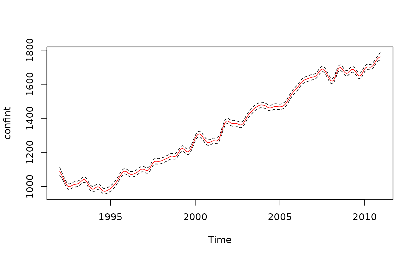
Let \((\theta_i)_{-p\leq i \leq q}\) be a moving average of length \(p+q+1\) used to filter a time series \((y_i)_{1\leq i \leq n}\). Let denote \(\hat{\mu}_t\) the filtered series computed at time \(t\) as: $$ \hat{\mu}_t = \sum_{i=-p}^q \theta_i y_{t+i}. $$ If \(\hat{\mu}_t\) is unbiased, a approximate confidence for the true mean is: $$ \left[\hat{\mu}_t - z_{1-\alpha/2} \hat{\sigma} \sqrt{\sum_{i=-p}^q\theta_i^2}; \hat{\mu}_t + z_{1-\alpha/2} \hat{\sigma} \sqrt{\sum_{i=-p}^q\theta_i^2} \right], $$ where \(z_{1-\alpha/2}\) is the quantile \(1-\alpha/2\) of the standard normal distribution.

The estimate of the variance \(\hat{\sigma}\) is obtained using var_estimator() with the parameter coef_var. The assumption that \(\hat{\mu}_t\) is unbiased is rarely exactly true, so variance estimates and confidence intervals are usually computed at small bandwidths where bias is small.

When coef (or coef_var) is a finite filter, the last points of the confidence interval are computed using the corresponding asymmetric filters

References

Loader, Clive. 1999. Local regression and likelihood. New York: Springer-Verlag.

Examples

x <- retailsa$DrinkingPlaces
coef <- lp_filter(6)
confint <- confint_filter(x, coef)
plot(confint, plot.type = "single",
     col = c("red", "black", "black"),
     lty = c(1, 2, 2))