Retrieve implicit forecasts corresponding to the asymmetric filters

Function to retrieve the implicit forecasts corresponding to the asymmetric filters

Usage

implicit_forecasts(x, coefs)

Arguments

x

a univariate or multivariate time series.

coefs

a matrix or a list that contains all the coefficients of the asymmetric and symmetric filters. (from the symmetric filter to the shortest). See details.

Details

Let \(h\) be the bandwidth of the symmetric filter, \(v_{-h}, \ldots, v_h\) the coefficients of the symmetric filter and \(w_{-h}^q, \ldots, w_h^q\) the coefficients of the asymmetric filter used to estimate the trend when \(q\) future values are known (with the convention \(w_{q+1}^q=\ldots=w_h^q=0\)). Let denote \(y_{-h},\ldots, y_0\) the last \(h\) available values of the input times series. The implicit forecast \(y_{1}^*,\dots y_h^*\) induced by \(w^0,\dots w^{h-1}\) are defined by: $$ \forall q\in\{0,...,h-1\}, \quad \sum_{i=-h}^0 v_iy_i + \sum_{i=1}^h v_iy_i^* =\sum_{i=-h}^0 w_i^qy_i + \sum_{i=1}^h w_i^qy_i^*. $$ which is equivalent to $$ \forall q, \sum_{i=1}^h (v_i- w_i^q) y_i^* =\sum_{i=-h}^0 (w_i^q-v_i)y_i. $$ Note that this is solved numerically: the solution isn't exact.

Examples

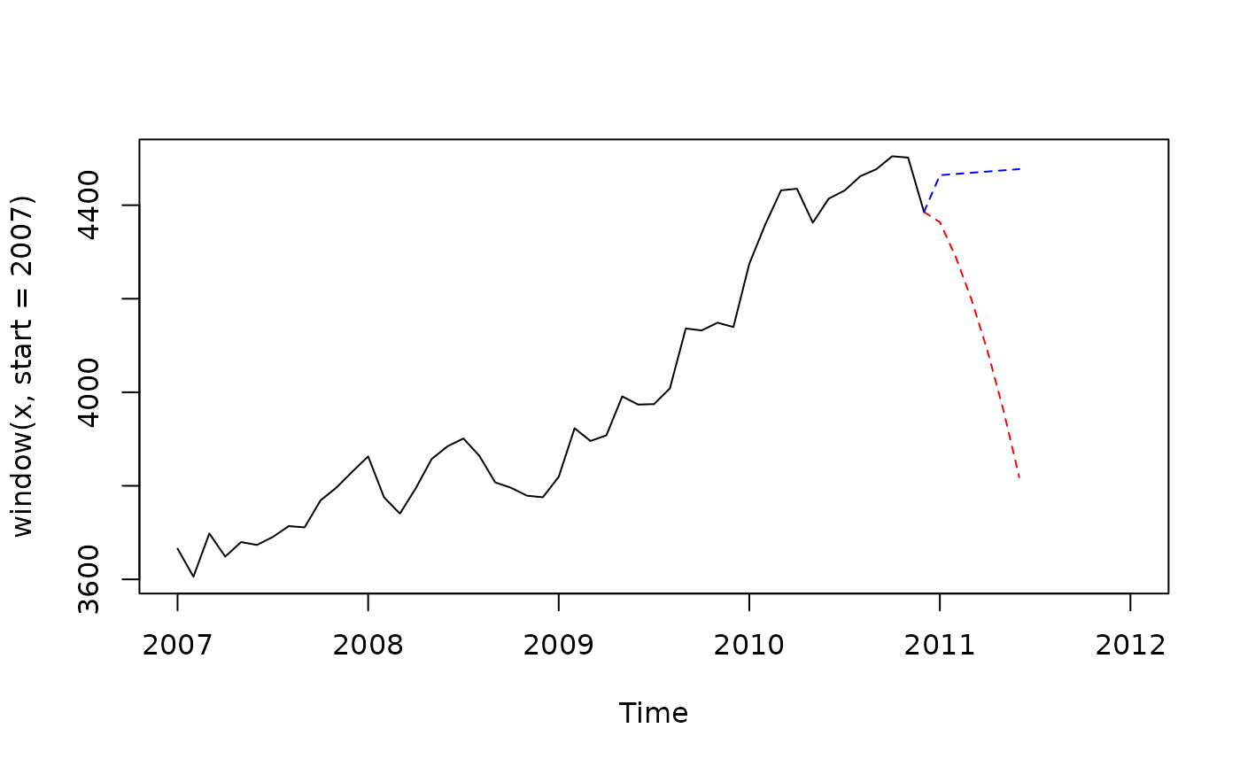
x <- retailsa$AllOtherGenMerchandiseStores
ql <- lp_filter(horizon = 6, kernel = "Henderson", endpoints = "QL")
lc <- lp_filter(horizon = 6, kernel = "Henderson", endpoints = "LC")
f_ql <- implicit_forecasts(x, ql)
f_lc <- implicit_forecasts(x, lc)

plot(window(x, start = 2007),
     xlim = c(2007,2012))
lines(ts(c(tail(x,1), f_ql), frequency = frequency(x), start = end(x)),
      col = "red", lty = 2)
lines(ts(c(tail(x,1), f_lc), frequency = frequency(x), start = end(x)),
      col = "blue", lty = 2)