Apply Local Polynomials Filters — localpolynomials • rjd3filters

Apply Local Polynomials Filters

Usage

localpolynomials(
  x,
  horizon = 6,
  degree = 3,
  kernel = c("Henderson", "Uniform", "Biweight", "Trapezoidal", "Triweight", "Tricube",
    "Gaussian", "Triangular", "Parabolic"),
  endpoints = c("LC", "QL", "CQ", "CC", "DAF"),
  ic = 3.5,
  tweight = 0,
  passband = pi/12
)

Arguments

x: input time-series.
horizon: horizon (bandwidth) of the symmetric filter.
degree: degree of polynomial.
kernel: kernel uses.
endpoints: method for endpoints.
ic: ic ratio.
tweight: timeliness weight.
passband: passband threshold.

Value

the target signal

References

Proietti, Tommaso and Alessandra Luati (2008). “Real time estimation in local polynomial regression, with application to trend-cycle analysis”.

See also

Examples

x <- retailsa$AllOtherGenMerchandiseStores
trend <- localpolynomials(x, horizon = 6)
#> Error in .jcall("jdplus/filters/base/r/LocalPolynomialFilters", "[D",     "filter", as.numeric(x), as.integer(horizon), as.integer(degree),     kernel, endpoints, d, tweight, passband): RcallMethod: cannot determine object class
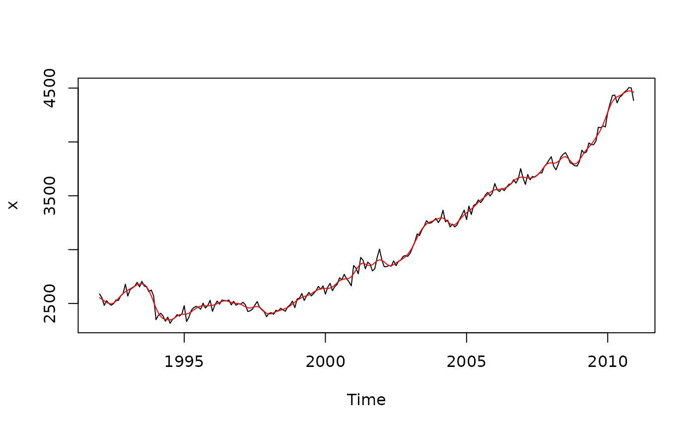
plot(x)

lines(trend, col = "red")
#> Error: object 'trend' not found