Plots filters properties

Functions to plot the coefficients, the gain and the phase functions.

Usage

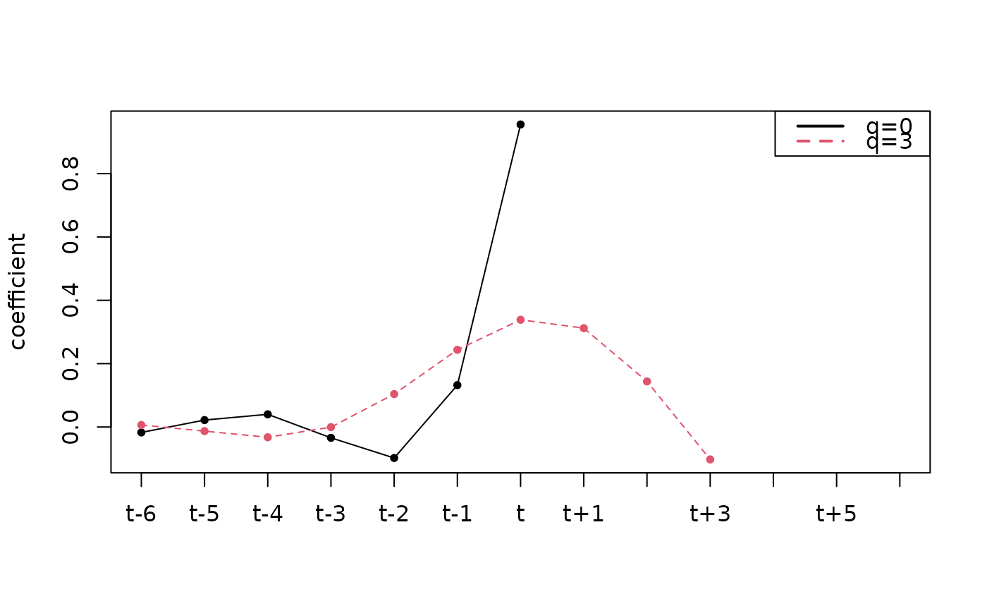
plot_coef(x, nxlab = 7, add = FALSE, ..., xlab = "", ylab = "coefficient")

# Default S3 method
plot_coef(
  x,
  nxlab = 7,
  add = FALSE,
  zero_as_na = TRUE,
  q = 0,
  legend = FALSE,
  legend.pos = "topright",
  ...,
  xlab = "",
  ylab = "coefficient"
)

# S3 method for class 'moving_average'
plot_coef(x, nxlab = 7, add = FALSE, ..., xlab = "", ylab = "coefficient")

# S3 method for class 'finite_filters'
plot_coef(
  x,
  nxlab = 7,
  add = FALSE,
  zero_as_na = TRUE,
  q = 0,
  legend = length(q) > 1,
  legend.pos = "topright",
  ...,
  xlab = "",
  ylab = "coefficient"
)

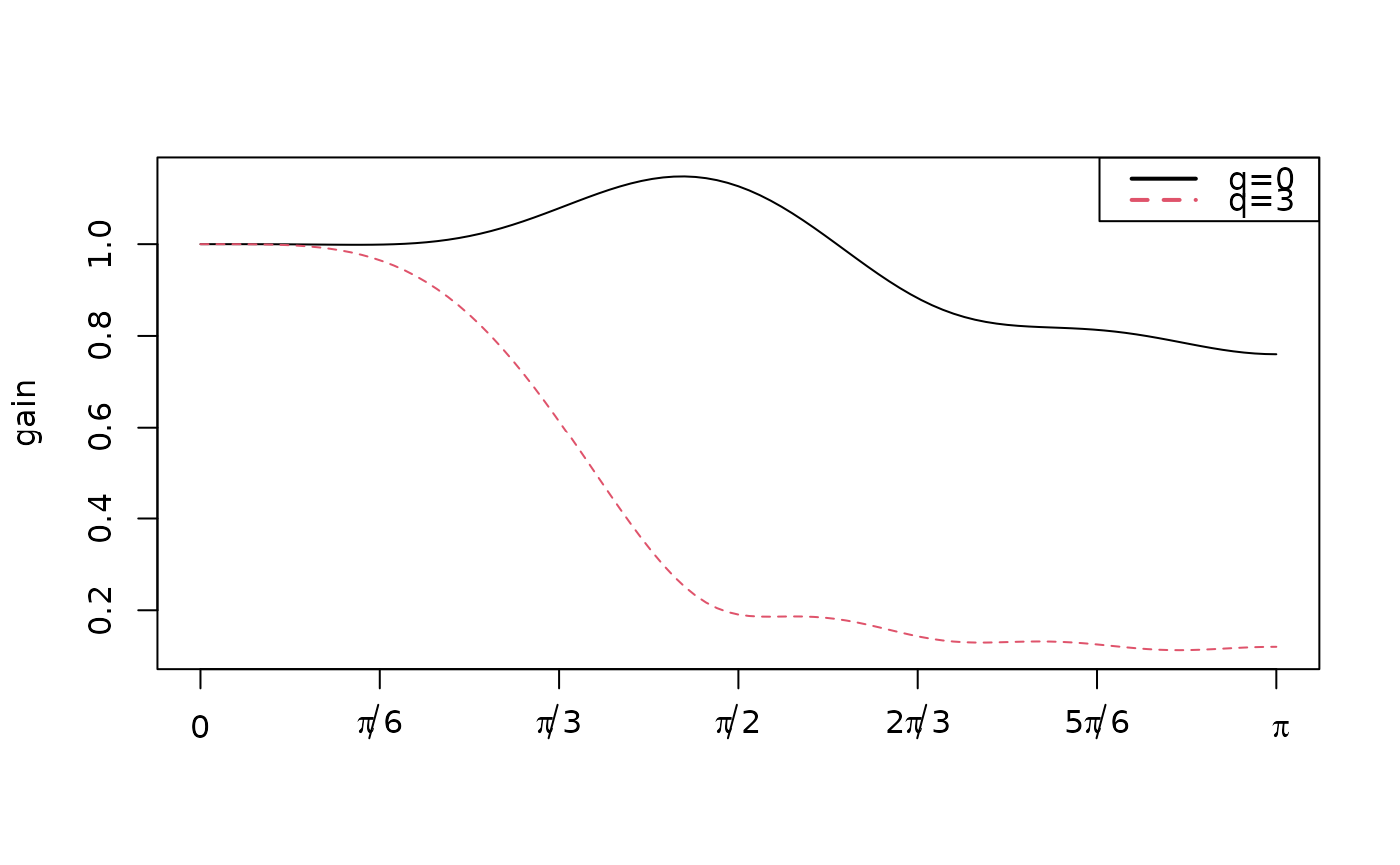
plot_gain(
  x,
  nxlab = 7,
  add = FALSE,
  xlim = c(0, pi),
  ...,
  xlab = "",
  ylab = "gain"
)

# S3 method for class 'moving_average'
plot_gain(
  x,
  nxlab = 7,
  add = FALSE,
  xlim = c(0, pi),
  ...,
  xlab = "",
  ylab = "gain"
)

# S3 method for class 'finite_filters'
plot_gain(
  x,
  nxlab = 7,
  add = FALSE,
  xlim = c(0, pi),
  q = 0,
  legend = length(q) > 1,
  legend.pos = "topright",
  n = 101,
  ...,
  xlab = "",
  ylab = "gain"
)

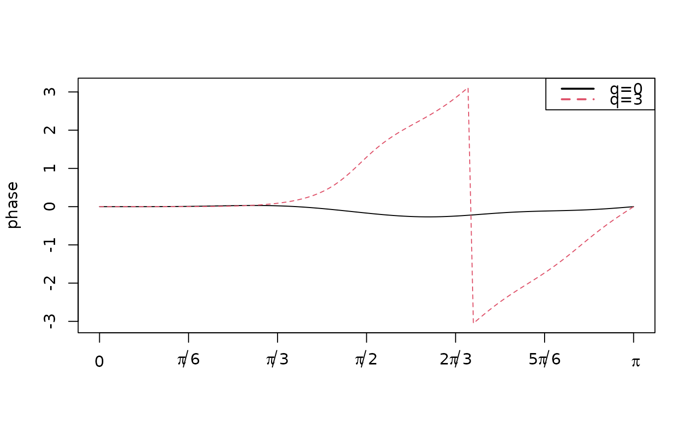
plot_phase(
  x,
  nxlab = 7,
  add = FALSE,
  xlim = c(0, pi),
  normalized = FALSE,
  ...,
  xlab = "",
  ylab = "phase"
)

# S3 method for class 'moving_average'
plot_phase(
  x,
  nxlab = 7,
  add = FALSE,
  xlim = c(0, pi),
  normalized = FALSE,
  ...,
  xlab = "",
  ylab = "phase"
)

# S3 method for class 'finite_filters'
plot_phase(
  x,
  nxlab = 7,
  add = FALSE,
  xlim = c(0, pi),
  normalized = FALSE,
  q = 0,
  legend = length(q) > 1,
  legend.pos = "topright",
  n = 101,
  ...,
  xlab = "",
  ylab = "phase"
)

Arguments

x

coefficients, gain or phase.

nxlab

number of xlab.

add

boolean indicating if the new plot is added to the previous one.

...

other arguments to matplot.

xlab, ylab

labels of axis.

zero_as_na

boolean indicating if the trailing zero of the coefficients should be plotted (FALSE) or removed (TRUE).

q

q.

legend

boolean indicating if the legend is printed.

legend.pos

position of the legend.

xlim

vector containing x limits.

n

number of points used to plot the functions.

normalized

boolean indicatif if the phase function is normalized by the frequency.

Examples

filter <- lp_filter(6, endpoints = "DAF", kernel = "Henderson")
#> Error in .jcall("jdplus/filters/base/r/LocalPolynomialFilters", "Ljdplus/toolkit/base/core/math/linearfilters/ISymmetricFiltering;",     "filters", as.integer(horizon), as.integer(degree), kernel,     endpoints, d, tweight, passband): java.lang.UnsupportedClassVersionError: jdplus/toolkit/base/core/math/linearfilters/IFiniteFilter has been compiled by a more recent version of the Java Runtime (class file version 65.0), this version of the Java Runtime only recognizes class file versions up to 61.0
plot_coef(filter, q = c(0,3), legend = TRUE)
#> Error in apply(x, 2, trailingzero_as_na): dim(X) must have a positive length
plot_gain(filter, q = c(0,3), legend = TRUE)
#> Error in UseMethod("plot_gain", x): no applicable method for 'plot_gain' applied to an object of class "function"
plot_phase(filter, q = c(0,3), legend = TRUE)
#> Error in UseMethod("plot_phase", x): no applicable method for 'plot_phase' applied to an object of class "function"