RegARIMA model, pre-adjustment in X13 and TRAMO-SEATS

The regarima/regarima_x13/regarima_tramoseats functions remove deterministic effects from the input series (e.g.calendar effects, outliers) using a multivariate regression model with arima errors. The jregarima/jregarima_x13/jregarima_tramoseats functions do the same computation but return the Java objects instead of a formatted output.

Usage

jregarima(series, spec = NA)

jregarima_tramoseats(
  series,
  spec = c("TRfull", "TR0", "TR1", "TR2", "TR3", "TR4", "TR5")
)

jregarima_x13(series, spec = c("RG5c", "RG0", "RG1", "RG2c", "RG3", "RG4c"))

regarima(series, spec = NA)

regarima_tramoseats(
  series,
  spec = c("TRfull", "TR0", "TR1", "TR2", "TR3", "TR4", "TR5")
)

regarima_x13(series, spec = c("RG5c", "RG0", "RG1", "RG2c", "RG3", "RG4c"))

Arguments

series

an univariate time series

spec

the model specification. For the function:

regarima: an object of class c("regarima_spec","X13") or c("regarima_spec","TRAMO_SEATS"). See the functions regarima_spec_x13 and regarima_spec_tramoseats.
regarima_x13: the name of a predefined X13 'JDemetra+' model specification (see Details). The default value is "RG5c".
regarima_tramoseats:the name of a predefined TRAMO-SEATS 'JDemetra+' model specification (see Details). The default value is "TRfull".

Value

The jregarima/jregarima_x13/jregarima_tramoseats functions return a jSA object that contains the result of the pre-adjustment method without any formatting. Therefore, the computation is faster than with the regarima/regarima_x13/regarima_tramoseats functions. The results of the seasonal adjustment can be extracted with the function get_indicators.

The regarima/regarima_x13/regarima_tramoseats functions return an object of class "regarima" and sub-class "X13" or "TRAMO_SEATS". regarima_x13 returns an object of class c("regarima","X13") and regarima_tramoseats, an object of class c("regarima","TRAMO_SEATS"). For the function regarima, the sub-class of the object depends on the used method that is defined by the spec object class.

An object of class "regarima" is a list containing the following components:

specification: a list with the model specification as defined by the spec argument. See also the Value of the regarima_spec_x13 and regarima_spec_tramoseats functions.
arma: a vector containing the orders of the autoregressive (AR), moving average (MA), seasonal AR and seasonal MA processes, as well as the regular and seasonal differencing orders (P,D,Q) (BP,BD,BQ).
arima.coefficients: a matrix containing the estimated regular and seasonal AR and MA coefficients, as well as the associated standard errors and t-statistics values. The estimated coefficients can be also extracted with the function coef (whose output also includes the regression coefficients).
regression.coefficients: a matrix containing the estimated regression variables (i.e.: mean, calendar effect, outliers and user-defined regressors) coefficients, as well as the associated standard errors and t-statistics values. The estimated coefficients can be also extracted with the function coef (whose output also includes the arima coefficients).
loglik: a matrix containing the log-likelihood of the RegARIMA model as well as the associated model selection criteria statistics (AIC, AICC, BIC and BICC) and parameters (np = number of parameters in the likelihood, neffectiveobs = number of effective observations in the likelihood). These statistics can also be extracted with the function logLik.
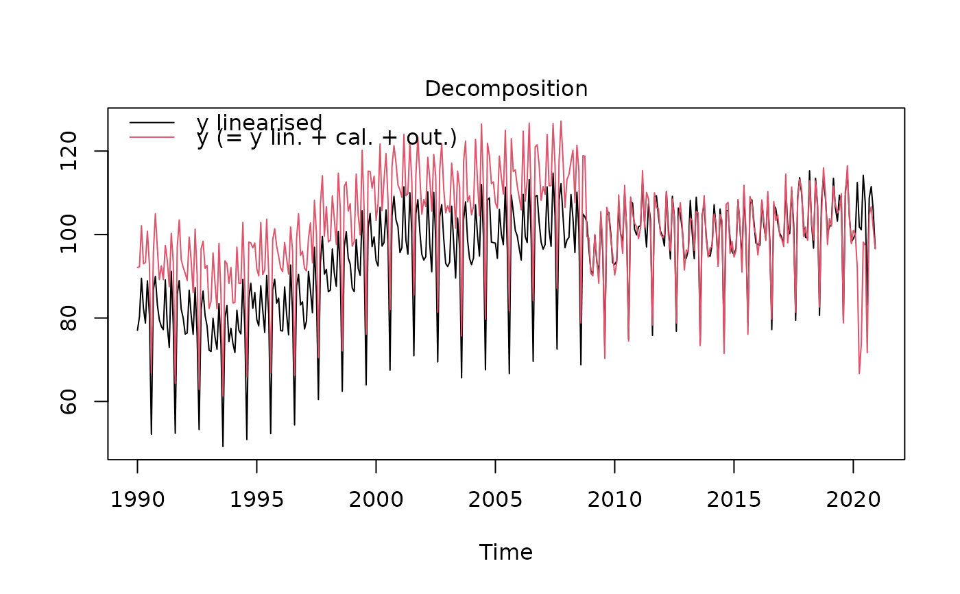
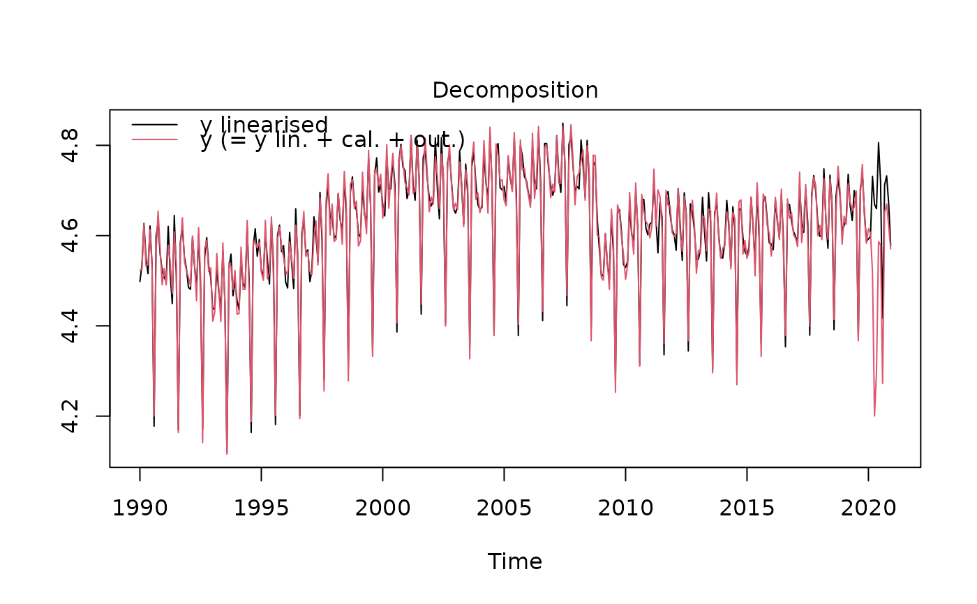
model: a list containing information on the model specification after its estimation (spec_rslt), as well as the decomposed elements of the input series (ts matrix, effects). The model specification includes information on the estimation method (Model) and time span (T.span), whether the original series was log transformed (Log transformation) and details on the regression part of the RegARIMA model i.e. if it includes a Mean, Trading days effects (if so, it provides the number of regressors), Leap year effect, Easter effect and whether outliers were detected (Outliers (if so, it provides the number of outliers). The decomposed elements of the input series contain the linearised series (y_lin) and the deterministic components i.e.: trading days effect (tde), Easter effect (ee), other moving holidays effect (omhe) and outliers effect (total - out, related to irregular - out_i, related to trend - out_t, related to seasonal - out_s).
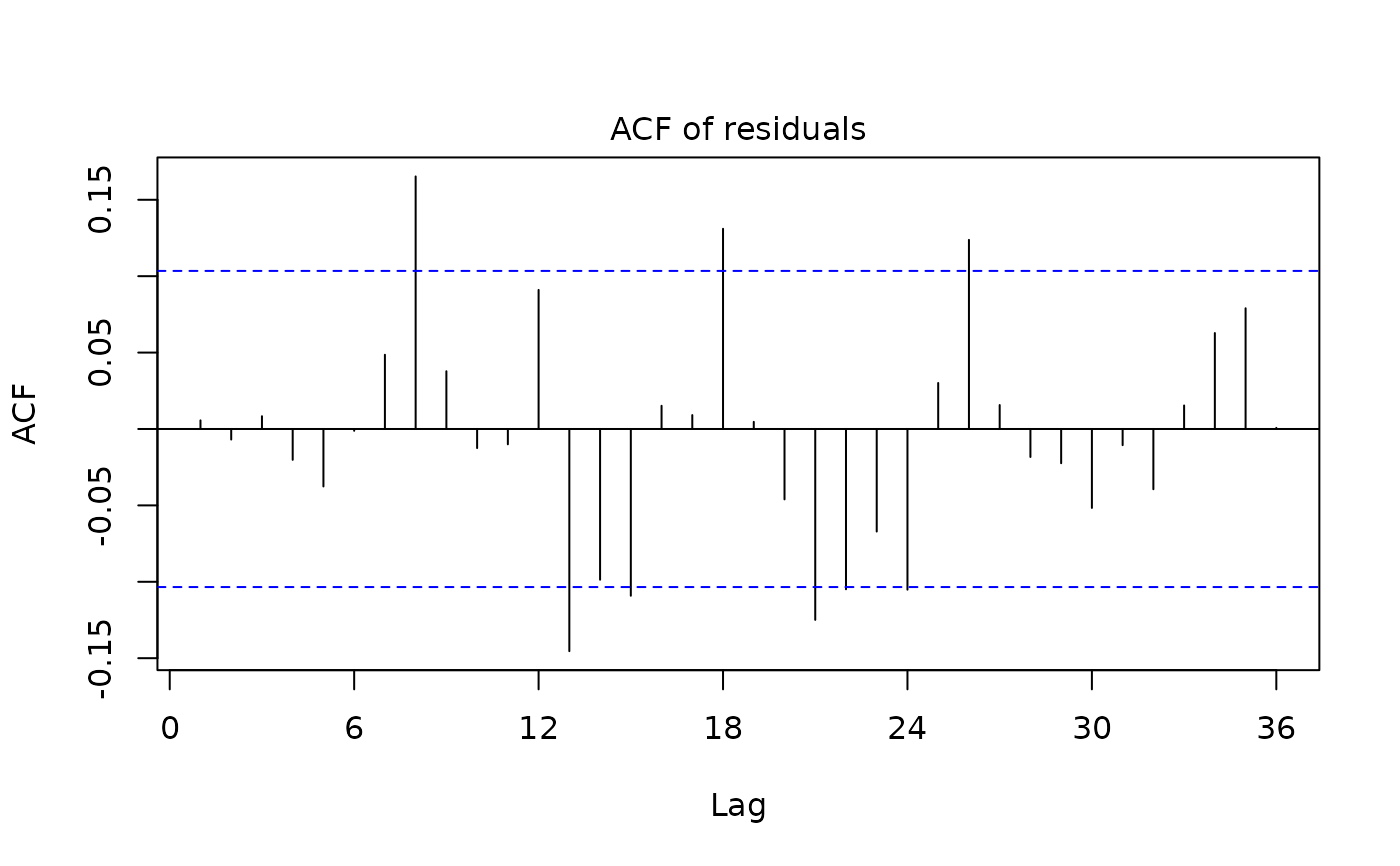
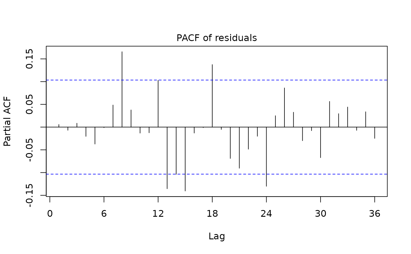
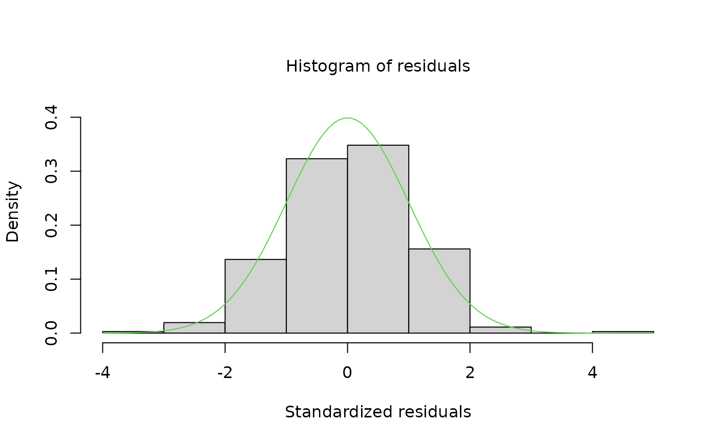
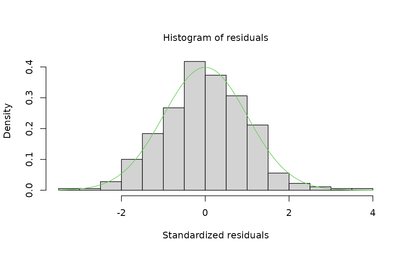
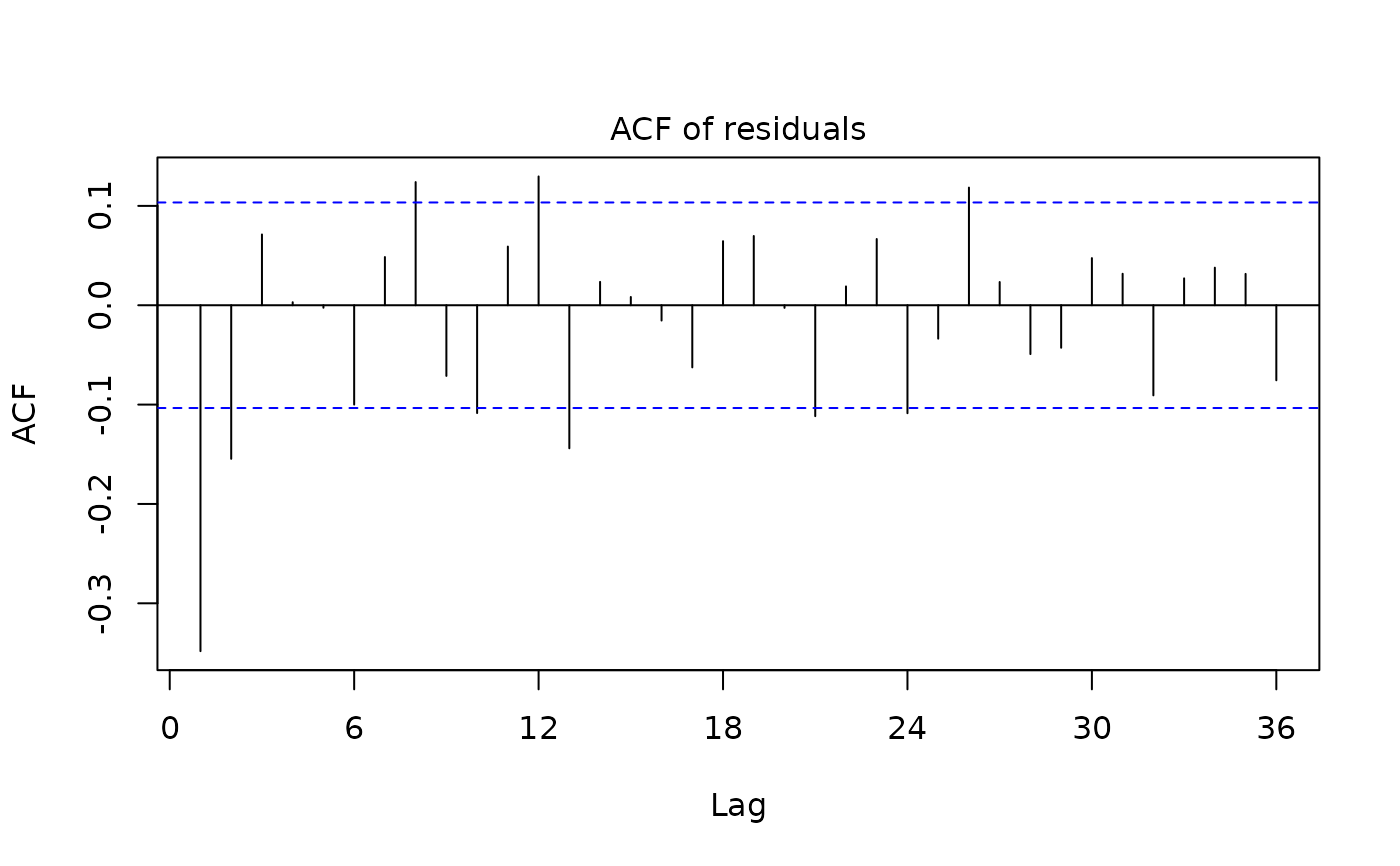
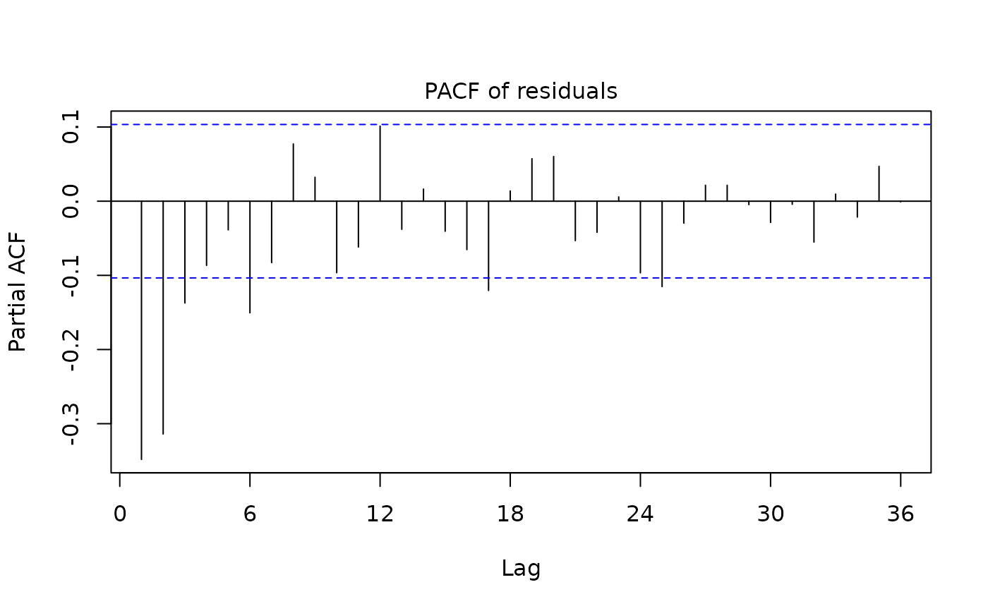
residuals: the residuals (time series). They can be also extracted with the function residuals.
residuals.stat: a list containing statistics on the RegARIMA residuals. It provides the residuals standard error (st.error) and the results of normality, independence and linearity of the residuals (tests) - object of class c("regarima_rtests","data.frame").
forecast: a ts matrix containing the forecast of the original series (fcst) and its standard error (fcsterr).

Details

When seasonally adjusting with X13 and TRAMO-SEATS, the first step consists in pre-adjusting the original series with a RegARIMA model, where the original series is corrected for any deterministic effects and missing observations. This step is also referred to as the linearization of the original series.

The RegARIMA model (model with ARIMA errors) is specified as such:

$$z_t = y_t\beta + x_t$$

where:

$z_t$ is the original series;
$\beta = (\beta_1,...,\beta_n)$ is a vector of regression coefficients;
$y_t = (y_{1t},...,y_{nt})$ are $n$ regression variables (outliers, calendar effects, user-defined variables);
$x_t$ is a disturbance that follows the general ARIMA process: $\phi(B)\delta(B)x_t = \theta(B)a_t$; where $\phi(B), \delta(B)$ and $\theta(B)$ are finite polynomials in $B$ and $a_t$ is a white noise variable with zero mean and a constant variance.

The polynomial $\phi(B)$ is a stationary autoregressive (AR) polynomial in $B$, which is a product of the stationary regular AR polynomial in $B$ and the stationary seasonal polynomial in $B^s$:

$$\phi(B)=\phi_p(B)\Phi_{bp}(B^s)=(1+\phi_1B+...+\phi_pB^p)(1+\Phi_1B^s+...+\Phi_{bp}B^{bps})$$

where:

$p$ is the number of regular AR terms (here and in 'JDemetra+', $p \le 3$);
$bp$ is the number of seasonal AR terms (here and in 'JDemetra+', $bp \le 1$);
$s$ is the number of observations per year (ie. The time series frequency).

The polynomial $\theta(B)$ is an invertible moving average (MA) polynomial in $B$, which is a product of the invertible regular MA polynomial in $B$ and the invertible seasonal MA polynomial in $B^s$:

$$\theta(B)=\theta_q(B)\Theta_{bq}(B^s)=(1+\theta_1B+...+\theta_qB^q)(1+\Theta_1B^s+...+\Theta_{bq}B^{bqs})$$

where:

$q$ is the number of regular MA terms (here and in 'JDemetra+', $q \le 3$);
$bq$ is the number of seasonal MA terms (here and in 'JDemetra+', $bq \le 1$).

The polynomial $\delta(B)$ is the non-stationary AR polynomial in $B$ (unit roots):

$$\delta(B) = (1-B)^d(1-B^s)^{d_s}$$

where:

$d$ is the regular differencing order (here and in 'JDemetra+', $d \le 1$);
$d_s$ is the seasonal differencing order (here and in 'JDemetra+', $d_s \le 1$).

NB. The notations used for AR and MA processes, as well as the model denoted as ARIMA $(P,D,Q)(BP,BD,BQ)$, are consistent with those in 'JDemetra+'.

The available predefined 'JDemetra+' X13 and TRAMO-SEATS model specifications are described in the tables below:

X13:

Identifier \|	Log/level detection \|	Outliers detection \|	Calendar effects \|	ARIMA	RG0 \|	NA \|
NA \|	NA \|	Airline(+mean)	RG1 \|	automatic \|	AO/LS/TC \|	NA \|
Airline(+mean)	RG2c \|	automatic \|	AO/LS/TC \|	2 td vars + Easter \|	Airline(+mean)	RG3 \|
automatic \|	AO/LS/TC \|	NA \|	automatic	RG4c \|	automatic \|	AO/LS/TC \|
2 td vars + Easter \|	automatic	RG5c \|	automatic \|	AO/LS/TC \|	7 td vars + Easter \|	automatic

TRAMO-SEATS:

Identifier \|	Log/level detection \|	Outliers detection \|	Calendar effects \|	ARIMA	TR0 \|	NA \|	NA \|
NA \|	Airline(+mean)	TR1 \|	automatic \|	AO/LS/TC \|	NA \|	Airline(+mean)	TR2 \|
automatic \|	AO/LS/TC \|	2 td vars + Easter \|	Airline(+mean)	TR3 \|	automatic \|	AO/LS/TC \|	NA \|
automatic	TR4 \|	automatic \|	AO/LS/TC \|	2 td vars + Easter \|	automatic	TR5 \|	automatic \|
AO/LS/TC \|	7 td vars + Easter \|	automatic	TRfull \|	automatic \|	AO/LS/TC \|	automatic \|	automatic

References

More information and examples related to 'JDemetra+' features in the online documentation: https://jdemetra-new-documentation.netlify.app/

BOX G.E.P. and JENKINS G.M. (1970), "Time Series Analysis: Forecasting and Control", Holden-Day, San Francisco.

BOX G.E.P., JENKINS G.M., REINSEL G.C. and LJUNG G.M. (2015), "Time Series Analysis: Forecasting and Control", John Wiley & Sons, Hoboken, N. J., 5th edition.

Examples

# \donttest{
 # X13 method
myseries <- ipi_c_eu[, "FR"]
myreg <- regarima_x13(myseries, spec ="RG5c")
summary(myreg)
#> y = regression model + arima (2, 1, 1, 0, 1, 1)
#> 
#> Model: RegARIMA - X13
#> Estimation span: from 1-1990 to 12-2020
#> Log-transformation: no
#> Regression model: no mean, trading days effect(7), leap year effect, Easter effect, outliers(4)
#> 
#> Coefficients:
#> ARIMA: 
#>             Estimate Std. Error  T-stat Pr(>|t|)    
#> Phi(1)     0.0003269  0.1077296   0.003   0.9976    
#> Phi(2)     0.1688192  0.0740996   2.278   0.0233 *  
#> Theta(1)  -0.5485606  0.1016550  -5.396 1.24e-07 ***
#> BTheta(1) -0.6660849  0.0422242 -15.775  < 2e-16 ***
#> ---
#> Signif. codes:  0 ‘***’ 0.001 ‘**’ 0.01 ‘*’ 0.05 ‘.’ 0.1 ‘ ’ 1
#> 
#> Regression model: 
#>               Estimate Std. Error  T-stat Pr(>|t|)    
#> Monday         0.55932    0.22801   2.453 0.014638 *  
#> Tuesday        0.88221    0.22832   3.864 0.000132 ***
#> Wednesday      1.03996    0.22930   4.535 7.85e-06 ***
#> Thursday       0.04943    0.22944   0.215 0.829549    
#> Friday         0.91132    0.22988   3.964 8.88e-05 ***
#> Saturday      -1.57769    0.22775  -6.927 1.99e-11 ***
#> Leap year      2.15403    0.70527   3.054 0.002425 ** 
#> Easter [1]    -2.37950    0.45391  -5.242 2.71e-07 ***
#> TC (4-2020)  -35.59245    2.17330 -16.377  < 2e-16 ***
#> AO (3-2020)  -20.89026    2.18013  -9.582  < 2e-16 ***
#> AO (5-2011)   13.49850    1.85694   7.269 2.28e-12 ***
#> LS (11-2008) -12.54901    1.63554  -7.673 1.60e-13 ***
#> ---
#> Signif. codes:  0 ‘***’ 0.001 ‘**’ 0.01 ‘*’ 0.05 ‘.’ 0.1 ‘ ’ 1
#> 
#> 
#> Residual standard error: 2.218 on 342 degrees of freedom
#> Log likelihood = -799.1, aic =  1632, aicc =  1634, bic(corrected for length) = 1.855
#> 
plot(myreg)







myspec1 <- regarima_spec_x13(myreg, tradingdays.option = "WorkingDays")
myreg1 <- regarima(myseries, myspec1)

myspec2 <- regarima_spec_x13(myreg, usrdef.outliersEnabled = TRUE,
             usrdef.outliersType = c("LS", "AO"),
             usrdef.outliersDate = c("2008-10-01", "2002-01-01"),
             usrdef.outliersCoef = c(36, 14),
             transform.function = "None")
myreg2 <- regarima(myseries, myspec2)
myreg2
#> y = regression model + arima (2, 1, 1, 0, 1, 1)
#> Log-transformation: no
#> Coefficients:
#>           Estimate Std. Error
#> Phi(1)     0.07859      0.114
#> Phi(2)     0.19792      0.076
#> Theta(1)  -0.48272      0.111
#> BTheta(1) -0.65916      0.043
#> 
#>               Estimate Std. Error
#> Monday         0.64094      0.228
#> Tuesday        0.81794      0.229
#> Wednesday      1.05374      0.229
#> Thursday       0.06981      0.228
#> Friday         0.93434      0.228
#> Saturday      -1.63686      0.226
#> Leap year      2.11550      0.697
#> Easter [1]    -2.38135      0.451
#> AO (9-2008)   31.95554      2.924
#> LS (9-2008)  -57.04093      2.657
#> TC (4-2020)  -35.62104      2.120
#> AO (3-2020)  -21.00931      2.145
#> AO (5-2011)   13.21877      1.832
#> TC (9-2008)   23.44654      4.001
#> TC (12-2001) -20.47521      2.922
#> AO (12-2001)  17.13461      2.962
#> TC (2-2002)   10.61731      1.937
#> 
#> Fixed outliers: 
#>              Coefficients
#> LS (10-2008)           36
#> AO (1-2002)            14
#> 
#> 
#> Residual standard error: 2.178 on 337 degrees of freedom
#> Log likelihood = -792.6, aic =  1629 aicc =  1632, bic(corrected for length) = 1.901
#> 

myspec3 <- regarima_spec_x13(myreg, automdl.enabled = FALSE,
             arima.p = 1, arima.q = 1,
             arima.bp = 0, arima.bq = 1,
             arima.coefEnabled = TRUE,
             arima.coef = c(-0.8, -0.6, 0),
             arima.coefType = c(rep("Fixed", 2), "Undefined"))
s_arimaCoef(myspec3)
#>                Type Value
#> Phi(1)        Fixed  -0.8
#> Theta(1)      Fixed  -0.6
#> BTheta(1) Undefined   0.0
myreg3 <- regarima(myseries, myspec3)
summary(myreg3)
#> y = regression model + arima (1, 1, 1, 0, 1, 1)
#> 
#> Model: RegARIMA - X13
#> Estimation span: from 1-1990 to 12-2020
#> Log-transformation: yes
#> Regression model: no mean, trading days effect(6), no leap year effect, Easter effect, outliers(3)
#> 
#> Coefficients:
#> ARIMA: 
#>           Estimate Std. Error T-stat Pr(>|t|)    
#> Phi(1)     -0.8000     0.0000     NA       NA    
#> Theta(1)   -0.6000     0.0000     NA       NA    
#> BTheta(1)  -0.6977     0.0399 -17.49   <2e-16 ***
#> ---
#> Signif. codes:  0 ‘***’ 0.001 ‘**’ 0.01 ‘*’ 0.05 ‘.’ 0.1 ‘ ’ 1
#> 
#> Regression model: 
#>              Estimate Std. Error  T-stat Pr(>|t|)    
#> Monday       0.006317   0.001791   3.526 0.000476 ***
#> Tuesday      0.007824   0.001793   4.363 1.68e-05 ***
#> Wednesday    0.010528   0.001802   5.841 1.16e-08 ***
#> Thursday     0.001857   0.001811   1.025 0.306022    
#> Friday       0.010099   0.001812   5.574 4.90e-08 ***
#> Saturday    -0.018439   0.001781 -10.354  < 2e-16 ***
#> Easter [1]  -0.020593   0.003515  -5.859 1.06e-08 ***
#> TC (4-2020) -0.475720   0.031229 -15.233  < 2e-16 ***
#> AO (3-2020) -0.213355   0.023246  -9.178  < 2e-16 ***
#> AO (5-2011)  0.143705   0.015529   9.254  < 2e-16 ***
#> ---
#> Signif. codes:  0 ‘***’ 0.001 ‘**’ 0.01 ‘*’ 0.05 ‘.’ 0.1 ‘ ’ 1
#> 
#> 
#> Residual standard error: 0.0256 on 347 degrees of freedom
#> Log likelihood = 802.3, aic =  1733, aicc =  1734, bic(corrected for length) = -7.15
#> 
plot(myreg3)







 # TRAMO-SEATS method
myspec <- regarima_spec_tramoseats("TRfull")
myreg <- regarima(myseries, myspec)
myreg
#> y = regression model + arima (2, 1, 0, 0, 1, 1)
#> Log-transformation: no
#> Coefficients:
#>           Estimate Std. Error
#> Phi(1)      0.4032      0.051
#> Phi(2)      0.2883      0.051
#> BTheta(1)  -0.6641      0.042
#> 
#>             Estimate Std. Error
#> Week days     0.6994      0.032
#> Leap year     2.3231      0.690
#> Easter [6]   -2.5154      0.436
#> AO (5-2011)  13.4679      1.787
#> TC (4-2020) -22.2128      2.205
#> TC (3-2020) -21.0391      2.217
#> AO (5-2000)   6.7386      1.794
#> 
#> 
#> Residual standard error: 2.326 on 348 degrees of freedom
#> Log likelihood = -816.1, aic =  1654 aicc =  1655, bic(corrected for length) = 1.852
#> 

myspec2 <- regarima_spec_tramoseats(myspec, tradingdays.mauto = "Unused",
             tradingdays.option = "WorkingDays",
             easter.type = "Standard",
             automdl.enabled = FALSE, arima.mu = TRUE)
myreg2 <- regarima(myseries, myspec2)

var1 <- ts(rnorm(length(myseries))*10, start = start(myseries), frequency = 12)
var2 <- ts(rnorm(length(myseries))*100, start = start(myseries), frequency = 12)
var <- ts.union(var1, var2)
myspec3 <- regarima_spec_tramoseats(myspec,
             usrdef.varEnabled = TRUE, usrdef.var = var)
s_preVar(myspec3)
#> $series
#>                  var1         var2
#> Jan 1990 -16.30989402    2.0831228
#> Feb 1990   5.12426950    0.7586777
#> Mar 1990 -18.63011492   93.0844030
#> Apr 1990  -5.22012515  -68.4749941
#> May 1990  -0.52601910   33.7401513
#> Jun 1990   5.42996343  -41.2137704
#> Jul 1990  -9.14074827   93.4261130
#> Aug 1990   4.68154420  184.0316741
#> Sep 1990   3.62951256  -70.4819663
#> Oct 1990 -13.04543545    0.8510312
#> Nov 1990   7.37776321  203.4189886
#> Dec 1990  18.88504929 -134.1686068
#> Jan 1991  -0.97445104  115.8979182
#> Feb 1991  -9.35847354  -20.3208958
#> Mar 1991  -0.15950311  -37.8028555
#> Apr 1991  -8.26788954  173.6111043
#> May 1991 -15.12399651  -84.5247816
#> Jun 1991   9.35363190  -96.1571493
#> Jul 1991   1.76488611  101.7491053
#> Aug 1991   2.43685465 -149.6053742
#> Sep 1991  16.23548883 -118.4818730
#> Oct 1991   1.12038083   63.0234373
#> Nov 1991  -1.33997013  210.1252514
#> Dec 1991 -19.10087468  -61.3736810
#> Jan 1992  -2.79237242 -163.4638272
#> Feb 1992  -3.13445978   -1.0441117
#> Mar 1992  10.67307879  -65.6506139
#> Apr 1992   0.70034850  -66.9533441
#> May 1992  -6.39123324  -47.8589028
#> Jun 1992  -0.49964899  131.9456316
#> Jul 1992  -2.51483443   63.6562761
#> Aug 1992   4.44797116   51.4327782
#> Sep 1992  27.55417575 -175.1375113
#> Oct 1992   0.46531380   89.3597518
#> Nov 1992   5.77709069   22.3038372
#> Dec 1992   1.18194874   58.0816593
#> Jan 1993 -19.11720491  -17.7821421
#> Feb 1993   8.62086482   74.0966708
#> Mar 1993  -2.43236740  -99.7443079
#> Apr 1993  -2.06087195 -293.8977561
#> May 1993   0.19177592   71.9015661
#> Jun 1993   0.29560754  -69.8005041
#> Jul 1993   5.49827542 -189.4125843
#> Aug 1993 -22.74114857    7.6299249
#> Sep 1993  26.82557184   87.5308501
#> Oct 1993  -3.61221255   45.3827393
#> Nov 1993   2.13355750  -85.0716906
#> Dec 1993  10.74345882   56.6201613
#> Jan 1994  -6.65088249  115.2211954
#> Feb 1994  11.13952419  -75.6197377
#> Mar 1994  -2.45896412  -48.9258334
#> Apr 1994 -11.77563309 -116.6052337
#> May 1994  -9.75850616  -47.9668950
#> Jun 1994  10.65057320   11.5348218
#> Jul 1994   1.31670635 -176.8048407
#> Aug 1994   4.88628809 -140.7638919
#> Sep 1994 -16.99450568   70.9178461
#> Oct 1994 -14.70736306 -124.0842940
#> Nov 1994   2.84150344  -36.8327348
#> Dec 1994  13.37320413   46.2080093
#> Jan 1995   2.36696283  -32.2833101
#> Feb 1995  13.18293384 -128.7214810
#> Mar 1995   5.23909788 -103.0040247
#> Apr 1995   6.06748047  151.4089316
#> May 1995  -1.09935672   34.6903586
#> Jun 1995   1.72181715  177.9441542
#> Jul 1995  -0.90327287   38.6630924
#> Aug 1995  19.24343341  -91.8695239
#> Sep 1995  12.98392759 -158.4336488
#> Oct 1995   7.48791268   -8.4058892
#> Nov 1995   5.56224329 -208.5070889
#> Dec 1995  -5.48257264    0.3567992
#> Jan 1996  11.10534893  -35.5770822
#> Feb 1996 -26.12334333  114.6359751
#> Mar 1996  -1.55693776  -22.1188446
#> Apr 1996   4.33889790  101.8179021
#> May 1996  -3.81951112  -26.3719295
#> Jun 1996   4.24187575  165.8542305
#> Jul 1996  10.63101996  -77.4086771
#> Aug 1996  10.48712620  -92.3937880
#> Sep 1996  -0.38102895  -27.5533378
#> Oct 1996   4.86148920  -59.3399688
#> Nov 1996  16.72882611  -12.2285891
#> Dec 1996  -3.54361164  117.9784246
#> Jan 1997   9.46347886   64.1037374
#> Feb 1997  13.16826356  -62.9588508
#> Mar 1997  -2.96640025  -80.7734971
#> Apr 1997  -3.87213575  -86.0489929
#> May 1997  -7.85432656 -216.9238693
#> Jun 1997 -10.56736867 -137.5836518
#> Jul 1997  -7.95541430  -49.3132472
#> Aug 1997 -17.56275428  -58.1652027
#> Sep 1997  -6.90537897  -16.7229304
#> Oct 1997  -5.58541994   48.5993129
#> Nov 1997  -5.36663326 -133.3395796
#> Dec 1997   2.27127133  -26.1965625
#> Jan 1998   9.78454920   65.2386303
#> Feb 1998  -2.08882651   74.8854971
#> Mar 1998 -13.99410460   89.6560285
#> Apr 1998   2.58537288  148.9300424
#> May 1998  -4.41799453  -65.9403481
#> Jun 1998   5.68599861   53.7283179
#> Jul 1998  21.26850459   74.6803067
#> Aug 1998   4.24858441  189.6317084
#> Sep 1998 -16.84281532 -206.0070725
#> Oct 1998   2.49401784    6.4543870
#> Nov 1998  10.72838252  -26.5147403
#> Dec 1998  20.39369263  -44.7344531
#> Jan 1999   4.49453778 -141.0700927
#> Feb 1999  13.91814046  -50.6418882
#> Mar 1999   4.26566547  -26.9761838
#> Apr 1999   1.07583992 -108.5154918
#> May 1999   0.22294733   36.2159127
#> Jun 1999   6.03611011  -33.5672143
#> Jul 1999  -2.62650573  136.3804498
#> Aug 1999  -5.28264082  -71.1524136
#> Sep 1999   1.92149422   66.2178797
#> Oct 1999 -11.46199669   29.1130223
#> Nov 1999   8.46184665   19.7958000
#> Dec 1999   0.81719629 -120.3566106
#> Jan 2000 -13.05117010   -3.9817044
#> Feb 2000  -9.44912060   68.6982465
#> Mar 2000   4.54341594   70.5267007
#> Apr 2000  -8.55202501   99.1441680
#> May 2000  -2.86895219  114.4248971
#> Jun 2000   8.94961626 -123.8910243
#> Jul 2000   0.67304440  265.4898333
#> Aug 2000  -1.62676337  -15.6917189
#> Sep 2000  -8.27310169  -42.3490117
#> Oct 2000  18.76505621  -19.8387058
#> Nov 2000   7.66440199  -89.4802407
#> Dec 2000   9.79956696   90.4269119
#> Jan 2001  13.21780992    7.9649210
#> Feb 2001 -11.19710829 -125.8827223
#> Mar 2001   5.14599819  102.5685106
#> Apr 2001 -15.09099836  -73.0778603
#> May 2001  15.32741480  -19.0145507
#> Jun 2001   4.29147371   52.8864693
#> Jul 2001   1.22103414   55.0210535
#> Aug 2001 -11.38012401   54.9684337
#> Sep 2001  -5.58015129  -65.9542372
#> Oct 2001  10.52538537    5.7421706
#> Nov 2001   6.77683644 -280.8010508
#> Dec 2001   0.38499547  -91.2259753
#> Jan 2002  -3.56381187  -78.2379163
#> Feb 2002   7.82844102  -66.4104924
#> Mar 2002   8.04411616   62.6309770
#> Apr 2002 -19.00060823  -50.7248206
#> May 2002   9.35784286   27.0361335
#> Jun 2002  -3.09051503   46.7476865
#> Jul 2002   2.63066677   72.3994958
#> Aug 2002 -17.90591856   61.3836939
#> Sep 2002  -7.88258845  -61.7869202
#> Oct 2002 -11.33021669   22.0724902
#> Nov 2002   3.63652568  112.7926598
#> Dec 2002  -2.85887914  181.3454336
#> Jan 2003   5.17669134   -8.3825685
#> Feb 2003  -1.02908670  136.7706666
#> Mar 2003  -9.74069593  -62.7434620
#> Apr 2003  12.70672301  -21.6629150
#> May 2003   9.60864787  -68.3713824
#> Jun 2003   7.68721370  -44.4702734
#> Jul 2003  10.35930771   60.6489806
#> Aug 2003  -4.73887074   62.4183075
#> Sep 2003 -12.75334875  -69.5431074
#> Oct 2003  -3.05620674  -78.3639078
#> Nov 2003  22.11769487  -95.3123859
#> Dec 2003 -10.41668381  179.2756071
#> Jan 2004 -11.46523850   34.8976696
#> Feb 2004 -16.75327303   25.9103768
#> Mar 2004  15.25938655  -80.5951897
#> Apr 2004   5.54185515   10.5664701
#> May 2004  19.93110265  -33.3599682
#> Jun 2004  -1.54120740  164.1847970
#> Jul 2004  25.64408338  -64.3905859
#> Aug 2004  10.61999145   58.7020562
#> Sep 2004  11.42694878  -15.0403088
#> Oct 2004  11.23838843 -171.0821848
#> Nov 2004  -3.97001493  143.1032558
#> Dec 2004  -8.23261151 -264.5212268
#> Jan 2005  -5.78884625 -103.2457405
#> Feb 2005  17.63789378  -70.7466431
#> Mar 2005   1.32992146  -70.0560014
#> Apr 2005   3.76499328   53.7885439
#> May 2005  11.38707653  -31.6332175
#> Jun 2005  12.41263075  -83.9622754
#> Jul 2005   6.12090945 -135.4928062
#> Aug 2005  -4.29380087  -81.7568272
#> Sep 2005  13.60461327  -63.4400003
#> Oct 2005  -0.70857431   81.5949433
#> Nov 2005  -2.72153684   30.2795706
#> Dec 2005 -24.46680029  180.7086625
#> Jan 2006   0.65486641  -89.4026756
#> Feb 2006 -10.98508902   -4.6428211
#> Mar 2006  -6.33178176  -47.1179138
#> Apr 2006 -20.63654451  -52.6692630
#> May 2006  26.48932029   -9.5134908
#> Jun 2006 -11.53398386 -249.5364809
#> Jul 2006  -3.40637876   16.6889217
#> Aug 2006   7.86362576   35.0492384
#> Sep 2006 -12.70513110  143.3701009
#> Oct 2006   5.42141549   76.5906803
#> Nov 2006   0.75105900  116.7520670
#> Dec 2006   5.58514422  -13.6943429
#> Jan 2007   4.15406399  -51.4902044
#> Feb 2007 -14.52299769  151.9744468
#> Mar 2007   9.41206122  -32.8491678
#> Apr 2007  -3.38935872   -5.3671506
#> May 2007  -0.75574247  -56.3524635
#> Jun 2007   0.40204392  -74.3908963
#> Jul 2007   1.24301066  -10.9041651
#> Aug 2007  -9.98432551  -56.0829227
#> Sep 2007  12.33390065   18.8001549
#> Oct 2007   3.40424488   74.8850942
#> Nov 2007  -4.72702482 -191.6538316
#> Dec 2007   7.08753061   23.6095847
#> Jan 2008 -15.28958715   62.8953415
#> Feb 2008   2.37425345   41.7925676
#> Mar 2008 -13.12814246  197.6758477
#> Apr 2008   7.47028587  -50.6286298
#> May 2008 -15.62518435 -110.9968853
#> Jun 2008   0.71053360  -94.8705723
#> Jul 2008  -6.39534770   47.6843757
#> Aug 2008  -8.45195739  -79.5201560
#> Sep 2008   6.75244698   23.4326923
#> Oct 2008  11.53375794 -122.2451097
#> Nov 2008 -16.86504742 -245.3647354
#> Dec 2008  -9.02814949 -148.9260814
#> Jan 2009  13.17633698  -43.2147734
#> Feb 2009  11.00189745  -94.2554006
#> Mar 2009  12.03767839  -12.1450799
#> Apr 2009 -14.31270777  133.6446798
#> May 2009  13.82910861  -86.0356182
#> Jun 2009   0.03125940   66.6537820
#> Jul 2009  -0.77886824 -142.1534746
#> Aug 2009   4.41428226  117.0056168
#> Sep 2009   1.28922896 -140.4714543
#> Oct 2009  -8.30214260  110.1708096
#> Nov 2009  -5.03592910   69.7986263
#> Dec 2009 -11.93641182  -86.4349803
#> Jan 2010  -7.51723323 -109.1470351
#> Feb 2010  14.55841403   -3.7051465
#> Mar 2010  -8.28603533   81.0053792
#> Apr 2010   2.89774460  -49.9355412
#> May 2010  -4.80053484   94.8031588
#> Jun 2010  -6.04829354  -17.4245957
#> Jul 2010  14.60110180 -110.6235952
#> Aug 2010   1.49679354  -94.5985005
#> Sep 2010 -14.33321100   28.9089591
#> Oct 2010  -0.10303319   87.6913145
#> Nov 2010  -2.12236035 -114.8903940
#> Dec 2010  -9.06340179 -113.7612756
#> Jan 2011 -21.02152479 -143.7246735
#> Feb 2011  18.93360464  -49.4143476
#> Mar 2011  -9.68125837   84.0801808
#> Apr 2011  -1.02603036   79.1534124
#> May 2011   2.39959572  -16.8848948
#> Jun 2011   0.60898893   61.2722104
#> Jul 2011 -21.77576028  -77.1158924
#> Aug 2011  -1.17860143   88.8628993
#> Sep 2011   1.12294787    1.3214477
#> Oct 2011   0.07886198   22.5339515
#> Nov 2011  18.77743872  -72.9915210
#> Dec 2011  21.58756554 -122.2487070
#> Jan 2012   7.09714522   40.6805171
#> Feb 2012   7.66983379  -75.1012223
#> Mar 2012  -3.08211421  -16.2116540
#> Apr 2012  10.12001849   35.2010126
#> May 2012  -9.19051597  -28.9058300
#> Jun 2012   5.63380077   10.4662227
#> Jul 2012   3.22482749   72.0186531
#> Aug 2012   3.66674363  -61.1046082
#> Sep 2012  11.29835153 -110.6914072
#> Oct 2012  -9.41498076   53.4803326
#> Nov 2012   2.17837643   73.6067968
#> Dec 2012  14.15412293 -122.2501574
#> Jan 2013  -3.83733048  102.1415310
#> Feb 2013  -1.74086374   46.5165158
#> Mar 2013  -2.21744517   79.0472705
#> Apr 2013 -10.09528722  -13.0264801
#> May 2013   4.80725266  -93.0285334
#> Jun 2013  16.04407328  -36.4851004
#> Jul 2013 -15.15024529   15.3872493
#> Aug 2013 -14.16023914   41.3154818
#> Sep 2013   8.76777327  248.0823360
#> Oct 2013   6.24132413 -217.9956742
#> Nov 2013  21.12277288   42.0874578
#> Dec 2013  -3.56124416  -35.7528325
#> Jan 2014 -10.64464209  -64.6861514
#> Feb 2014  10.77116538   -5.0141801
#> Mar 2014  11.81575567   41.6942847
#> Apr 2014   1.98392095  -63.2587542
#> May 2014  -4.00405249  115.0146673
#> Jun 2014   6.16154281  -23.5475907
#> Jul 2014  19.74156748 -164.3107386
#> Aug 2014  18.84662324 -150.3382146
#> Sep 2014 -15.88620547 -205.0584847
#> Oct 2014  -5.39923164  -75.3198229
#> Nov 2014 -11.69461464  -13.4141958
#> Dec 2014   5.59105989  100.5782847
#> Jan 2015 -18.19347247  216.7186798
#> Feb 2015   3.93343972  232.2556540
#> Mar 2015   0.42134106 -102.0423391
#> Apr 2015  11.79664177    4.8814436
#> May 2015  -2.56921176  -77.1888628
#> Jun 2015 -10.56336098  -78.5235068
#> Jul 2015   1.98777205  -72.6603031
#> Aug 2015   6.50533552   68.1878032
#> Sep 2015   3.43913337  -22.9843287
#> Oct 2015  14.77532312 -151.0601724
#> Nov 2015   0.72025698  -58.3727687
#> Dec 2015  21.26444534 -202.2918454
#> Jan 2016 -14.76196906   40.3504676
#> Feb 2016   4.07888500   55.0015549
#> Mar 2016  13.93977798    2.8357122
#> Apr 2016   3.60278296   89.3165020
#> May 2016   6.54550251  -37.6555496
#> Jun 2016  10.52155422   60.5884808
#> Jul 2016 -19.79555125   -0.4874726
#> Aug 2016  12.08385605  -52.0796373
#> Sep 2016  -1.69280084  -63.9018598
#> Oct 2016   2.95029753  -63.5894137
#> Nov 2016  12.66340587   10.6586975
#> Dec 2016 -11.35343257  117.6914248
#> Jan 2017 -11.31053798   44.7391153
#> Feb 2017   1.09993384  227.2954766
#> Mar 2017   8.52905410   13.6058206
#> Apr 2017  -2.34337862 -199.9039133
#> May 2017  20.86688567  -42.0500870
#> Jun 2017  -1.10919371  -37.8407395
#> Jul 2017 -13.92847056  122.0774789
#> Aug 2017 -11.42290768 -154.1030292
#> Sep 2017  17.04608737  -31.0310122
#> Oct 2017  -0.80073634   -2.0108184
#> Nov 2017  -4.37281240 -239.0200336
#> Dec 2017  -1.19215094   88.9865359
#> Jan 2018   7.86462865 -148.2813325
#> Feb 2018  -5.78945246   44.5750348
#> Mar 2018  -1.45426885  136.9775856
#> Apr 2018   5.26457991   -2.0110027
#> May 2018  17.33578110  -10.9217587
#> Jun 2018  14.48657220   26.4661745
#> Jul 2018  15.18193149   30.3848264
#> Aug 2018  -3.84007254  -18.3388483
#> Sep 2018  18.27125177   55.9649672
#> Oct 2018  -5.51491750  -18.6553842
#> Nov 2018  -8.65753541  -81.2275372
#> Dec 2018  -3.43831481 -164.0581672
#> Jan 2019  10.62876458   50.7922478
#> Feb 2019   8.13058204  175.4336961
#> Mar 2019  18.03483361   59.2400202
#> Apr 2019  -1.05068694  101.6713288
#> May 2019   9.82453362   12.1620586
#> Jun 2019 -17.13302622 -107.8067265
#> Jul 2019  -8.32019527 -114.3565720
#> Aug 2019  11.00491882  -52.9643677
#> Sep 2019  -1.73820106  -68.1273156
#> Oct 2019   1.78812018  -20.2447559
#> Nov 2019  -6.98429449  168.4495721
#> Dec 2019  -9.60449159 -103.3773237
#> Jan 2020  -9.75423042  -15.5976673
#> Feb 2020  -3.38576503   -4.6400637
#> Mar 2020  11.52347074  -95.3628727
#> Apr 2020   4.05101183   41.6260798
#> May 2020  -4.70922497   11.4029609
#> Jun 2020  -1.33251019    6.3918753
#> Jul 2020  12.26682356  -91.9332238
#> Aug 2020   3.32943995   90.1335290
#> Sep 2020  -3.47088466  -79.7728297
#> Oct 2020  -0.98550690   66.8221204
#> Nov 2020   0.34766060   15.5214296
#> Dec 2020   3.86127022   12.8688092
#> 
#> $description
#>           type coeff
#> var1 Undefined    NA
#> var2 Undefined    NA
#> 
myreg3 <- regarima(myseries, myspec3)
myreg3
#> y = regression model + arima (2, 1, 0, 1, 1, 1)
#> Log-transformation: no
#> Coefficients:
#>           Estimate Std. Error
#> Phi(1)      0.4744      0.051
#> Phi(2)      0.3312      0.051
#> BPhi(1)    -0.2569      0.072
#> BTheta(1)  -0.8066      0.043
#> 
#>               Estimate Std. Error
#> r.var1        0.016274      0.009
#> r.var2        0.001222      0.001
#> Week days     0.689237      0.036
#> Leap year     2.054858      0.662
#> Easter [6]   -2.509781      0.411
#> TC (4-2020) -22.552758      2.120
#> TC (3-2020) -21.119937      2.128
#> AO (5-2011)  12.809939      1.739
#> LS (1-2009)  -9.611835      1.796
#> 
#> 
#> Residual standard error: 2.244 on 345 degrees of freedom
#> Log likelihood = -803.6, aic =  1635 aicc =  1636, bic(corrected for length) = 1.829
#> 
# }

Identifier \|	Log/level detection \|	Outliers detection \|	Calendar effects \|	ARIMA	RG0 \|	NA \|
NA \|	NA \|	Airline(+mean)	RG1 \|	automatic \|	AO/LS/TC \|	NA \|
Airline(+mean)	RG2c \|	automatic \|	AO/LS/TC \|	2 td vars + Easter \|	Airline(+mean)	RG3 \|
automatic \|	AO/LS/TC \|	NA \|	automatic	RG4c \|	automatic \|	AO/LS/TC \|
2 td vars + Easter \|	automatic	RG5c \|	automatic \|	AO/LS/TC \|	7 td vars + Easter \|	automatic

Identifier \|	Log/level detection \|	Outliers detection \|	Calendar effects \|	ARIMA	TR0 \|	NA \|	NA \|
NA \|	Airline(+mean)	TR1 \|	automatic \|	AO/LS/TC \|	NA \|	Airline(+mean)	TR2 \|
automatic \|	AO/LS/TC \|	2 td vars + Easter \|	Airline(+mean)	TR3 \|	automatic \|	AO/LS/TC \|	NA \|
automatic	TR4 \|	automatic \|	AO/LS/TC \|	2 td vars + Easter \|	automatic	TR5 \|	automatic \|
AO/LS/TC \|	7 td vars + Easter \|	automatic	TRfull \|	automatic \|	AO/LS/TC \|	automatic \|	automatic