Linear Filtering on a Time Series

Applies linear filtering to a univariate time series or to each series separately of a multivariate time series using either a moving average (symmetric or asymmetric) or a combination of symmetric moving average at the center and asymmetric moving averages at the bounds.

Usage

filter(x, coefs, remove_missing = TRUE)

Arguments

x

a univariate or multivariate time series.

coefs

a matrix or a list that contains all the coefficients of the asymmetric and symmetric filters. (from the symmetric filter to the shortest). See details.

remove_missing

if TRUE (default) leading and trailing NA are removed before filtering.

Details

The functions filter extends filter allowing to apply every kind of moving averages (symmetric and asymmetric filters) or to apply aset multiple moving averages to deal with the boundaries.

Let \(x_t\) be the input time series to filter.

• If coef is an object moving_average(), of length \(q\), the result \(y\) is equal at time \(t\) to: $$y[t] = x[t-lags] * coef[1] + x[t-lags+1] * coef[1] + ... + x[t-lags+q] * coef[q]$$. It extends the function filter that would add NA at the end of the time series.

• If coef is a matrix, list or finite_filters() object, at the center, the symmetric moving average is used (first column/element of coefs). At the boundaries, the last moving average of coefs is used to compute the filtered time series \(y[n]\) (no future point known), the second to last to compute the filtered time series \(y[n-1]\) (one future point known)...

Examples

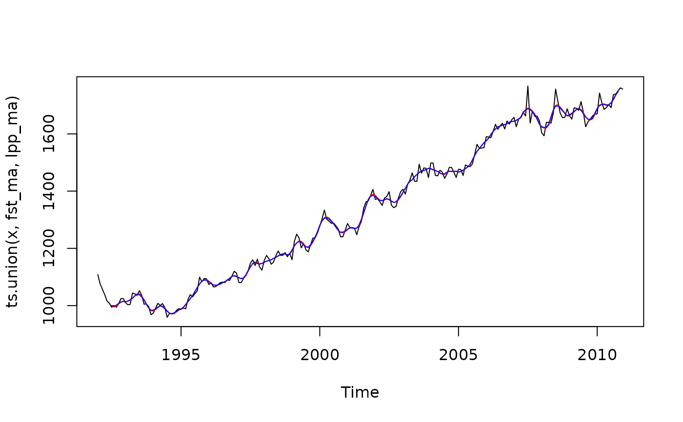
x <- retailsa$DrinkingPlaces

lags <- 6
leads <- 2
fst_coef <- fst_filter(lags = lags, leads = leads, smoothness.weight = 0.3, timeliness.weight = 0.3)
lpp_coef <- lp_filter(horizon = lags, kernel = "Henderson", endpoints = "LC")

fst_ma <- filter(x, fst_coef)
lpp_ma <- filter(x, lpp_coef[,"q=2"])

plot(ts.union(x, fst_ma, lpp_ma), plot.type = "single", col = c("black","red","blue"))


trend <- filter(x, lpp_coef)
# This is equivalent to:
trend <- localpolynomials(x, horizon = 6)