rjd3highfreq provides functions for seasonal adjustment of high-frequency data displaying multiple, non integer periodicities. Pre-adjustment with extended airline model and Arima Model Based decomposition.
Installation
Running rjd3 packages requires Java 17 or higher. How to set up such a configuration in R is explained here
Latest release
To get the current stable version (from the latest release):
- From GitHub:
# install.packages("remotes")
remotes::install_github("rjdverse/rjd3highfreq@*release")- From r-universe:
install.packages("rjd3highfreq", repos = c("https://rjdverse.r-universe.dev", "https://cloud.r-project.org"))Development version
You can install the development version of rjd3highfreq from GitHub with:
# install.packages("remotes")
remotes::install_github("rjdverse/rjd3highfreq")
Demonstration with the daily french births
## Import of data
df_daily <- read.csv2("https://raw.githubusercontent.com/TanguyBarthelemy/Tsace_RJD_Webinar_Dec22/b5fcf6b14ae47393554950547ef4788a0068a0f6/Data/TS_daily_births_franceM_1968_2020.csv")

# Creation of log variables to multiplicative model
df_daily$log_births <- log(df_daily$births)
df_daily$date <- as.Date(df_daily$date)
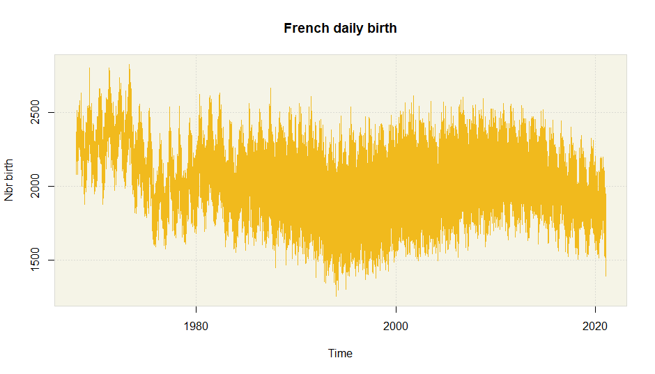
Plot of the raw series:
Preparation of the calendar with the package rjd3toolkit:
# French calendar
frenchCalendar <- rjd3toolkit::national_calendar(days = list(
  rjd3toolkit::fixed_day(7, 14), # Bastille Day
  rjd3toolkit::fixed_day(5, 8, validity = list(start = "1982-05-08")), # End of 2nd WW
  rjd3toolkit::special_day('NEWYEAR'),
  rjd3toolkit::special_day('MAYDAY'), # 1st may
  rjd3toolkit::special_day('EASTERMONDAY'),
  rjd3toolkit::special_day('ASCENSION'),
  rjd3toolkit::special_day('WHITMONDAY'),
  rjd3toolkit::special_day('ASSUMPTION'),
  rjd3toolkit::special_day('ALLSAINTSDAY'), # Toussaint
  rjd3toolkit::special_day('ARMISTICE'), # End of 1st WW
  rjd3toolkit::special_day('CHRISTMAS'))
)
Creation of the calendar regressor in a matrix with the package rjd3toolkit:
# Calendar regressor matrix
cal_reg <- rjd3toolkit::holidays(
    calendar = frenchCalendar,
    start = "1968-01-01", length = nrow(df_daily),
    type = "All", nonworking = 7L)

colnames(cal_reg) <- c("14th_july", "8th_may", "1st_jan", "1st_may",
                       "east_mon", "asc", "pen_mon",
                       "15th_aug", "1st_nov", "11th_nov", "Xmas")
Preprocessing with the function fractionalAirlineEstimation:
pre_pro <- fractionalAirlineEstimation(
    y = df_daily$births,
    x = cal_reg,
    periods = 7, # weekly frequency
    outliers = c("ao", "wo"), log = TRUE, y_time = df_daily$date)

print(pre_pro)
#> Number of observations: 19359
#> Start: 1968-01-01
#> End: 2020-12-31
#>
#> Estimate MA parameters:
#>       MA_parameter      Coef     Coef_SE    Tstat
#>           Theta(1) 0.7620698 0.005571472 136.7807
#>  Theta(period = 7) 0.9731793 0.001413477 688.5002
#>
#> Number of calendar regressors: 11 , Number of outliers : 7
#>
#> TD regressors coefficients:
#>   Variable    Coef Coef_SE    Tstat
#>  14th_july -0.1226  0.0047 -26.0615
#>    8th_may -0.1419  0.0054 -26.3419
#>    1st_jan -0.2223  0.0047 -47.3511
#>    1st_may -0.1225  0.0047 -26.2643
#>   east_mon -0.1891  0.0046 -40.7635
#>        asc -0.1726  0.0046 -37.1949
#>    pen_mon -0.1900  0.0046 -40.9429
#>   15th_aug -0.1181  0.0047 -25.3461
#>    1st_nov -0.1503  0.0046 -32.5662
#>   11th_nov -0.1238  0.0046 -26.8142
#>       Xmas -0.2310  0.0046 -49.7435
#>
#> Outliers coefficients:
#>       Variable    Coef Coef_SE   Tstat
#>  WO.1999-12-31 -0.1762  0.0226 -7.7916
#>  AO.1995-08-15 -0.2224  0.0340 -6.5503
#>  WO.1999-12-24 -0.1447  0.0226 -6.3981
#>  AO.2012-01-01  0.2098  0.0340  6.1786
#>  AO.1998-07-14 -0.2101  0.0340 -6.1880
#>  AO.1997-07-14 -0.2092  0.0340 -6.1602
#>  AO.1995-05-01 -0.2042  0.0340 -6.0146
#>
#> Sum of square residuals: 25.17 on 19330 degrees of freedom
#> Log likelihood = 3.682e+04,
#>  aic = -7.361e+04,
#>  aicc = -7.361e+04,
#>  bic(corrected for length) = -6.635
#> Hannan–Quinn information criterion = -7.355e+04
plot(pre_pro, main = "French births")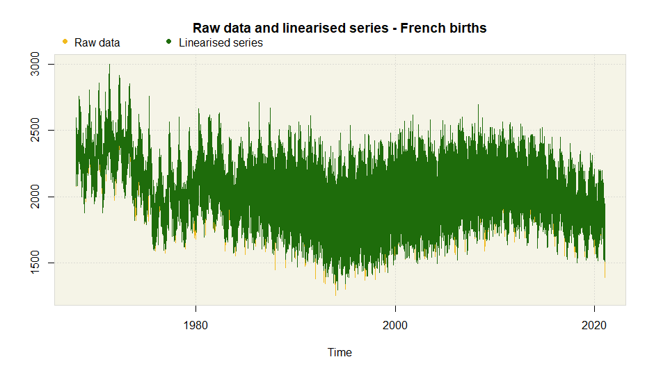
plot(x = pre_pro,
     from = as.Date("2000-01-01"), to = as.Date("2000-12-31"),
     main = "French births in 2000")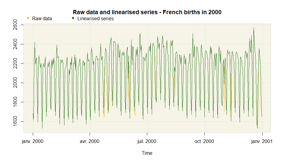
Decomposition with the AMB (Arima Model Based) algorithm:
# Decomposition with weekly pattern
amb.dow <- rjd3highfreq::fractionalAirlineDecomposition(
    y = pre_pro$model$linearized, # linearized series from preprocessing
    period = 7,
    log = TRUE, y_time = df_daily$date)

# Extract day-of-year pattern from day-of-week-adjusted linearised data
amb.doy <- rjd3highfreq::fractionalAirlineDecomposition(
    y = amb.dow$decomposition$sa, # DOW-adjusted linearised data
    period = 365.2425, # day of year pattern
    log = TRUE, y_time = df_daily$date)
Plot:
plot(amb.dow, main = "Weekly pattern")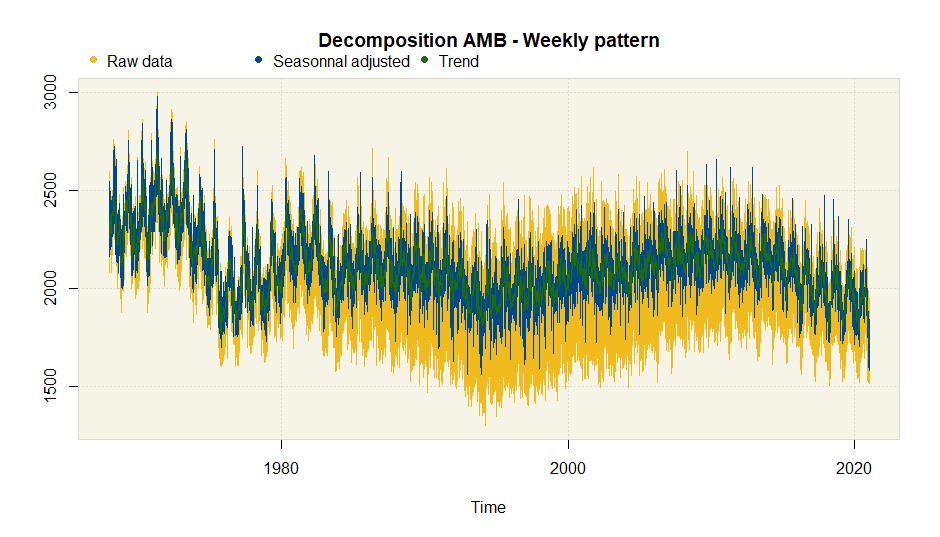
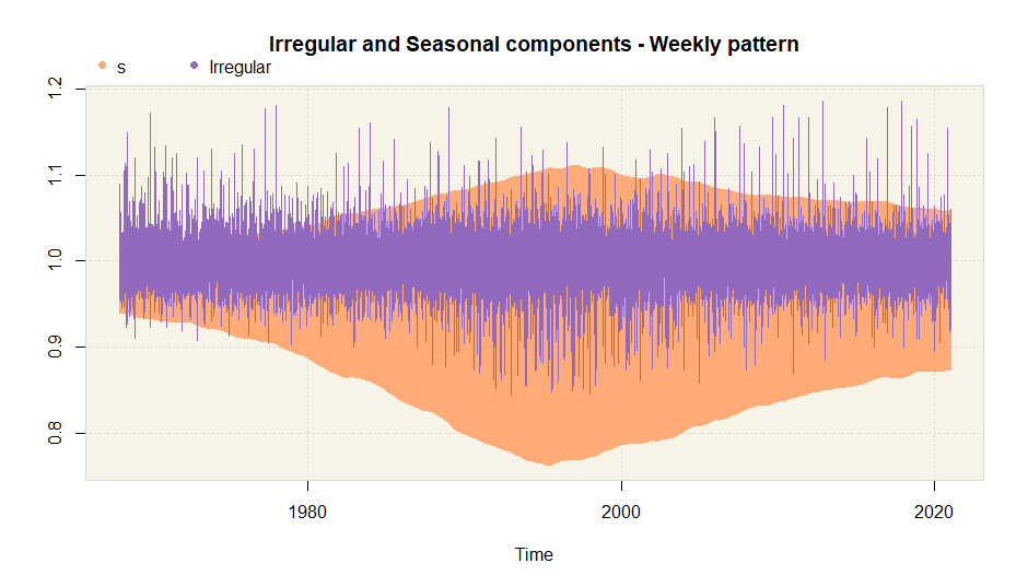
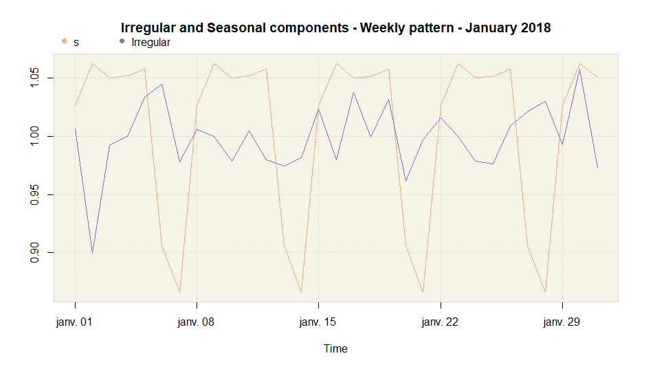
plot(amb.dow, main = "Weekly pattern - January 2018",
     from = as.Date("2018-01-01"),
     to = as.Date("2018-01-31"))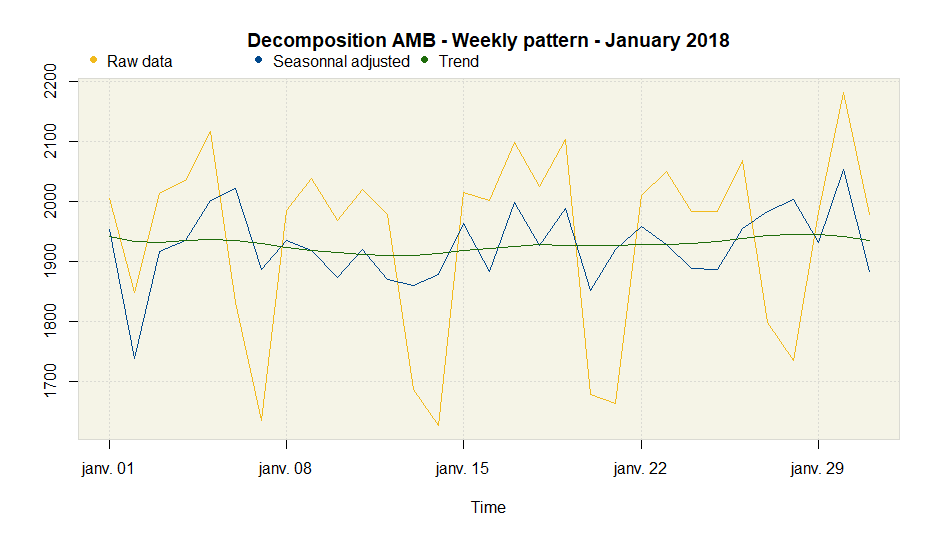
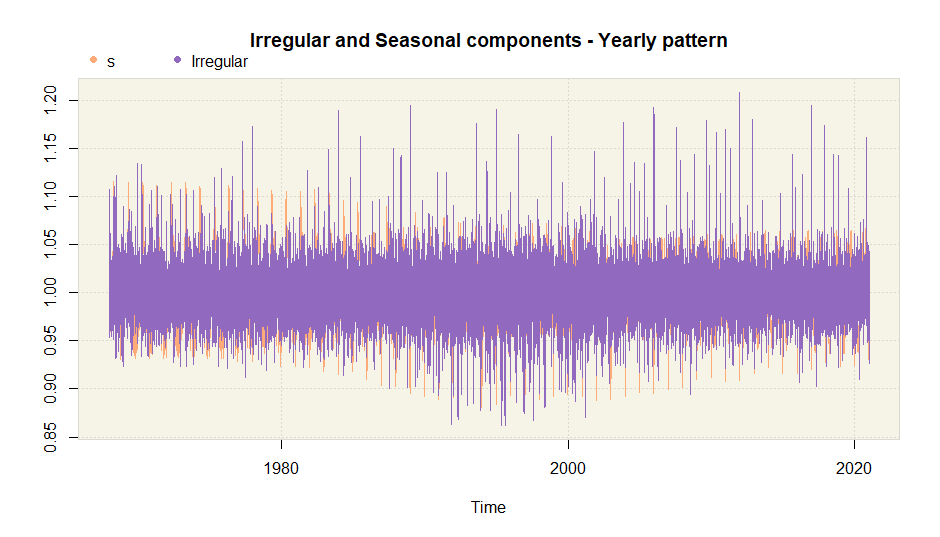
plot(amb.doy, main = "Yearly pattern")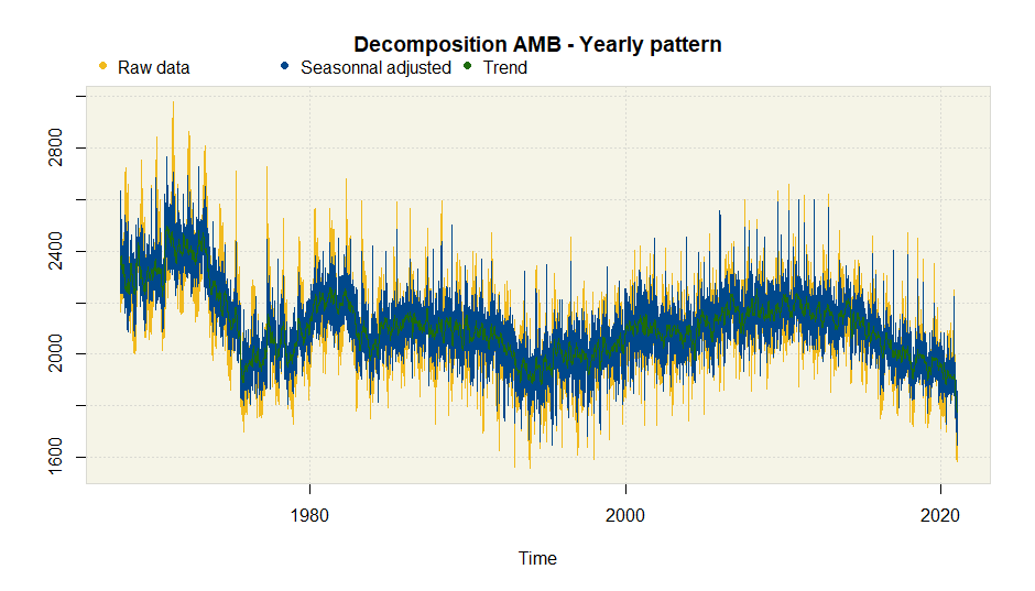
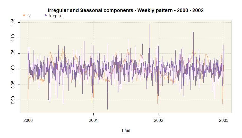
plot(amb.doy, main = "Weekly pattern - 2000 - 2002",
     from = as.Date("2000-01-01"),
     to = as.Date("2002-12-31"))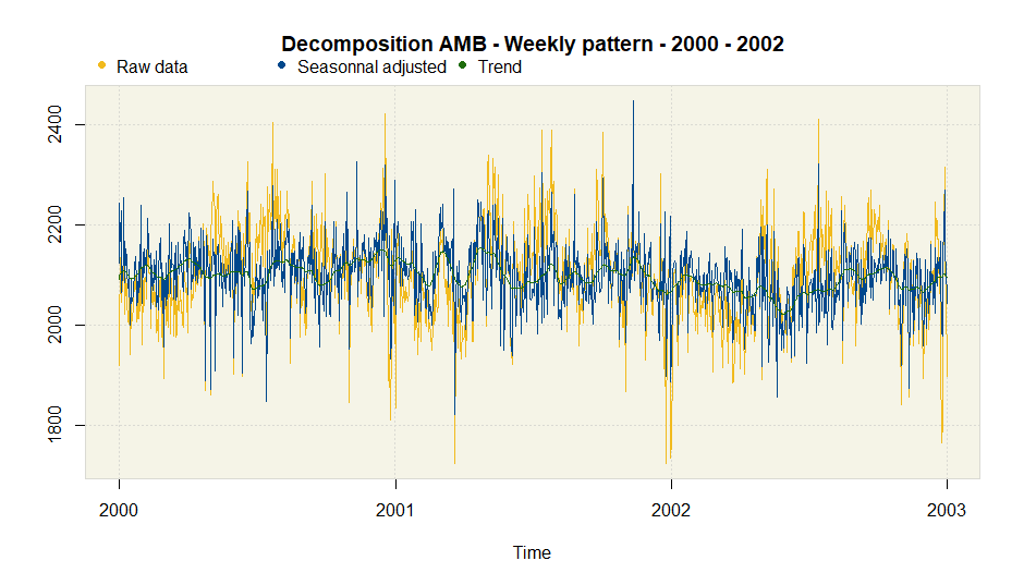
Perform an Arima Model Based (AMB) decomposition on several periodcities at once:
amb.multi <- rjd3highfreq::multiAirlineDecomposition(
  y = pre_pro$model$linearized, # input time series
  periods = c(7, 365.2425), # 2 frequency
  log = TRUE, y_time = df_daily$date)
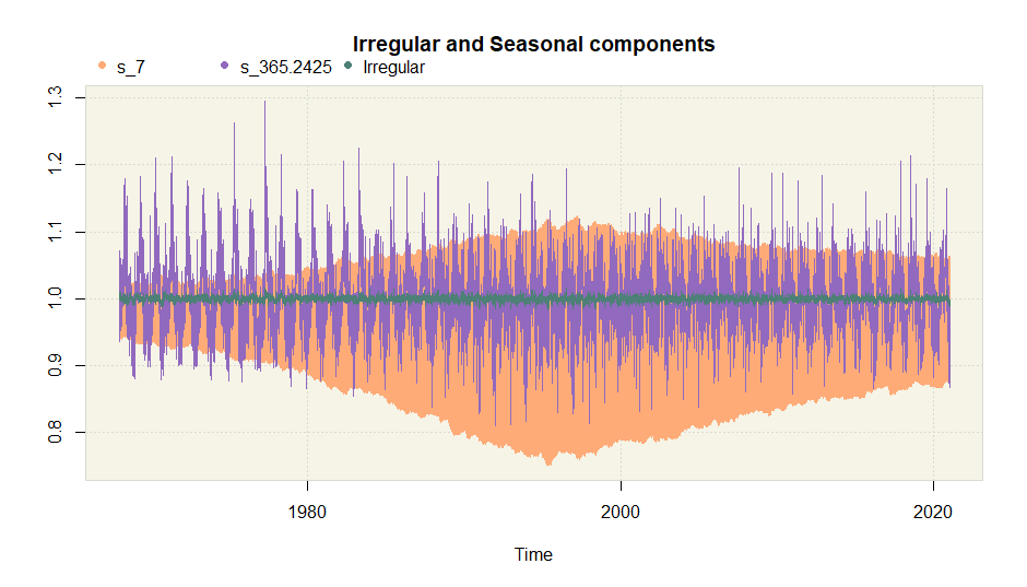
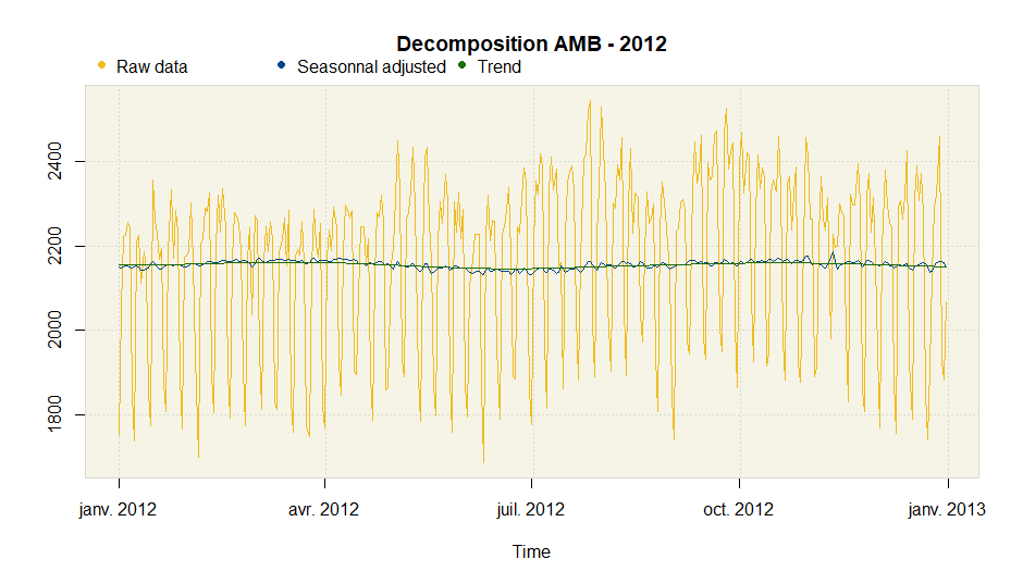
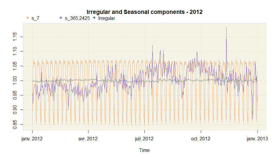
Plot the comparison between the two AMB methods for the annual periodicity:
plot(amb.multi)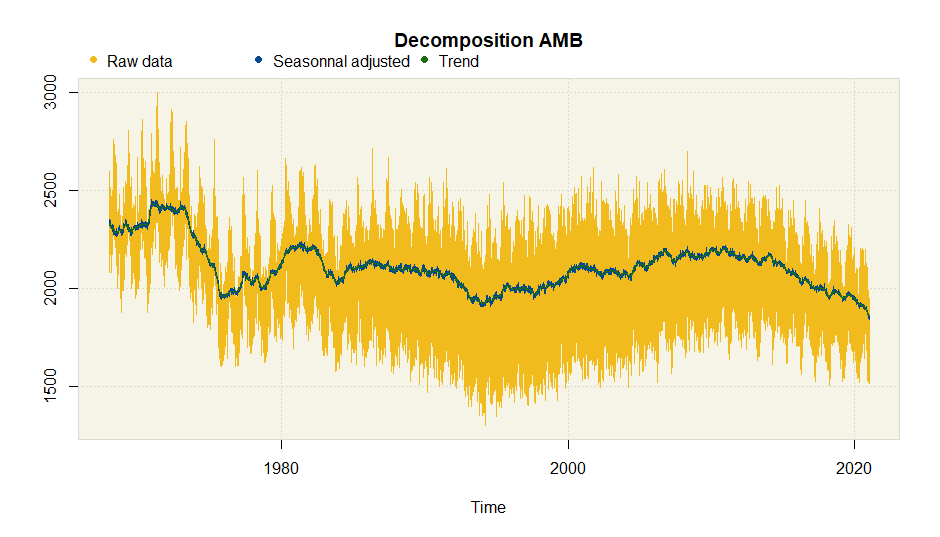
With the package rjd3x11plus, you can perform an X-11 like decomposition with any (non integer) periodicity.
Package Maintenance and contributing
Any contribution is welcome and should be done through pull requests and/or issues. pull requests should include updated tests and updated documentation. If functionality is changed, docstrings should be added or updated.
Licensing
The code of this project is licensed under the European Union Public Licence (EUPL).