BSM

Jean Palate

2024-07-12

Defining a Basic Structural Model with rjd3sts

The package allows several equivalent definitions of a basic structural model. We present below some of them.

To compare the results (more precisely the likelihood) of the different approaches, it is important to compute the marginal likelihood.

s<-log(retail$BookStores)

Standard definition, noise in the state

# create the model
bsm<-model()
# create the components and add them to the model
add(bsm, locallineartrend("ll"))
add(bsm, seasonal("s", 12, type="HarrisonStevens"))
add(bsm, noise("n"))
rslt<-estimate(bsm, log(s), marginal=TRUE)

• Likelihood = 747.8184945
• Parameters = 0.160016, 0.000396, 0.243922, 1.000000

Standard definition, noise in the measurement

# create the model
bsm<-model()
# create the components and add them to the model
add(bsm, locallineartrend("ll"))
add(bsm, seasonal("s", 12, type="HarrisonStevens"))
  # create the equation (fix the variance to 1)
eq<-equation("eq", 1,TRUE)
add_equation(eq, "ll")
add_equation(eq, "s")
add(bsm, eq)
rslt<-estimate(bsm, log(s), marginal=TRUE)

• Likelihood = 747.8184945
• Parameters = 0.160016, 0.000396, 0.243922, 1.000000

components with fixed variances, aggregated with diffuse weights (noise in the state)

# create the model
bsm<-model()
  # create the components, with fixed variances, and add them to the model
add(bsm, locallineartrend("ll", 
                             levelVariance = 1, fixedLevelVariance = TRUE) )
add(bsm, seasonal("s", 12, type="HarrisonStevens", 
                     variance = 1, fixed = TRUE))
add(bsm, noise("n", 1, fixed=TRUE))
  # create the equation (fix the variance to 1)
eq<-equation("eq", 0, TRUE)
add_equation(eq, "ll", .01, FALSE)
add_equation(eq, "s", .01, FALSE)
add_equation(eq, "n")
add(bsm, eq)
rslt<-estimate(bsm, log(s), marginal=TRUE)
p<-result(rslt, "parameters")

• Likelihood = 747.8184944
• Parameters = 1.0000, 0.0025, 1.0000, 1.0000, 0.4001, 0.4939

To be noted:

• Level variance = $p[5]\times p[5]$ = 0.160057
• Slope variance = $p[5]\times p[5] \times p[2]$ = 0.000396
• Seas variance = $p[6]\times p[6]$ = 0.243976

bsm with long term trend and cycle

# create the model
bsm<-model()
  # create the components and add them to the model
add(bsm, locallevel("l", initial = 0) )
add(bsm, locallineartrend("lt", levelVariance = 0, 
                             fixedLevelVariance = TRUE) )
add(bsm, seasonal("s", 12, type="HarrisonStevens"))
add(bsm, noise("n", 1, fixed=TRUE))
  # create the equation (fix the variance to 1)
rslt<-estimate(bsm, log(s), marginal=TRUE)

• Likelihood = 747.8184945
• Parameters = 0.160016, 0.000000, 0.000396, 0.243922, 1.000000

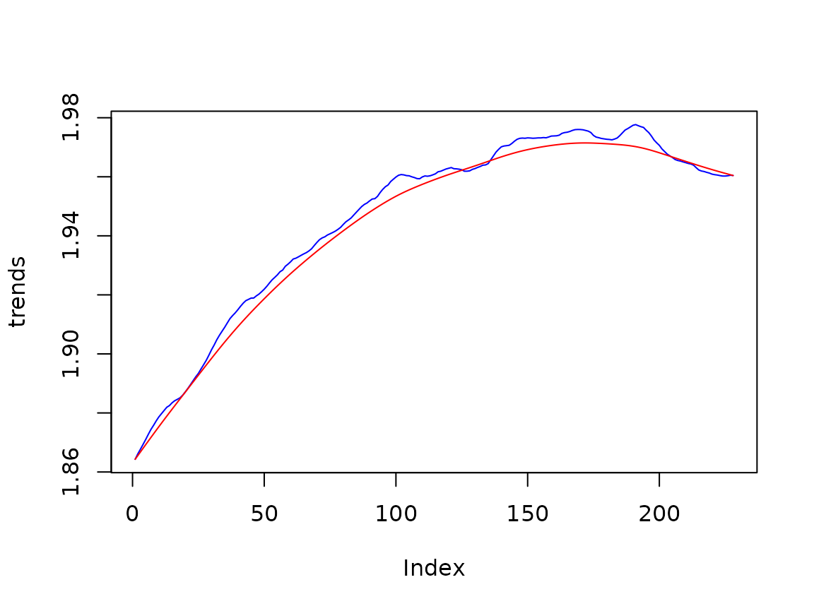
ss<-smoothed_states(rslt)
plot(ss[,1]+ss[,2], type='l', col='blue', ylab='trends')
lines(ss[, 2], col='red')