Functions to estimate the seasonally adjusted series (sa) with the TRAMO-SEATS method.
This is achieved by decomposing the time series (y) into the trend-cycle (t), the seasonal component (s) and the irregular component (i).
Calendar-related movements can be corrected in the pre-treatment (TRAMO) step.
tramoseats returns a preformatted result while jtramoseats returns the Java objects of the seasonal adjustment.
Arguments
- series
an univariate time series
- spec
a TRAMO-SEATS model specification. It can be the name (
character) of a pre-defined TRAMO-SEATS 'JDemetra+' model specification (see Details), or an object of classc("SA_spec","TRAMO_SEATS"). The default value is"RSAfull".- userdefined
a
charactervector containing the additional output variables (seeuser_defined_variables).
Value
jtramoseats returns a jSA object that contains the results of the seasonal adjustment without
any formatting. Therefore, the computation is faster than with the function tramoseats. The results of the seasonal
adjustment can be extracted with the function get_indicators.
tramoseats returns an object of class c("SA","TRAMO_SEATS"), that is, a list containing :
- regarima
an object of class
c("regarima","TRAMO_SEATS"). More info in the Value section of the functionregarima.- decomposition
an object of class
"decomposition_SEATS", that is a five-element list:specificationa list with the SEATS algorithm specification. See also the functiontramoseats_spec.modethe decomposition modemodelthe SEATS model list:model, sa, trend, seasonal, transitory, irregular, each element being a matrix of estimated coefficients.linearizedthe time series matrix (mts) with the stochastic series decomposition (input seriesy_lin, seasonally adjusted seriessa_lin, trendt_lin, seasonals_lin, irregulari_lin)componentsthe time series matrix (mts) with the decomposition components (input seriesy_cmp, seasonally adjusted seriessa_cmp, trendt_cmp, seasonal components_cmp, irregulari_cmp)
- final
an object of class
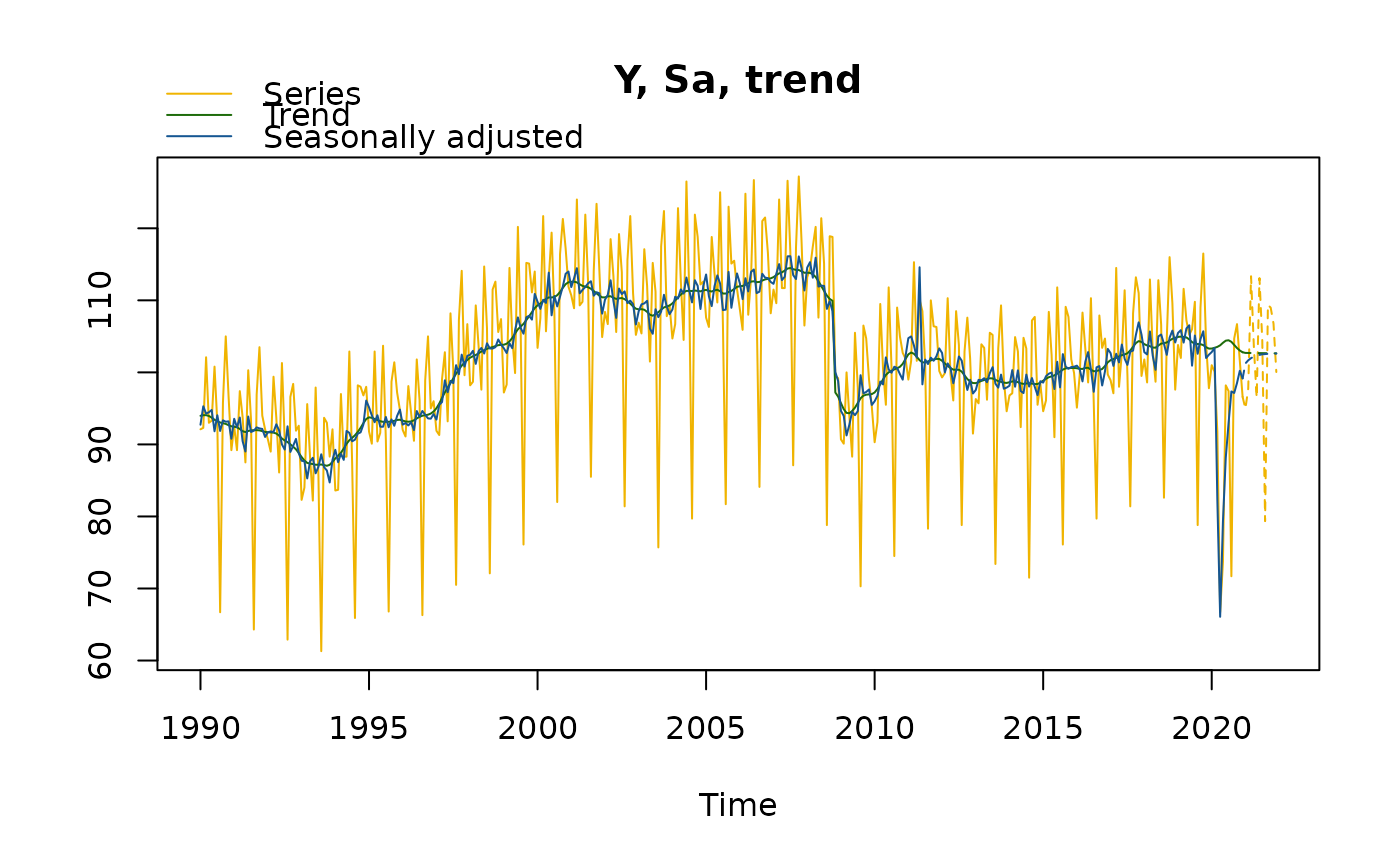
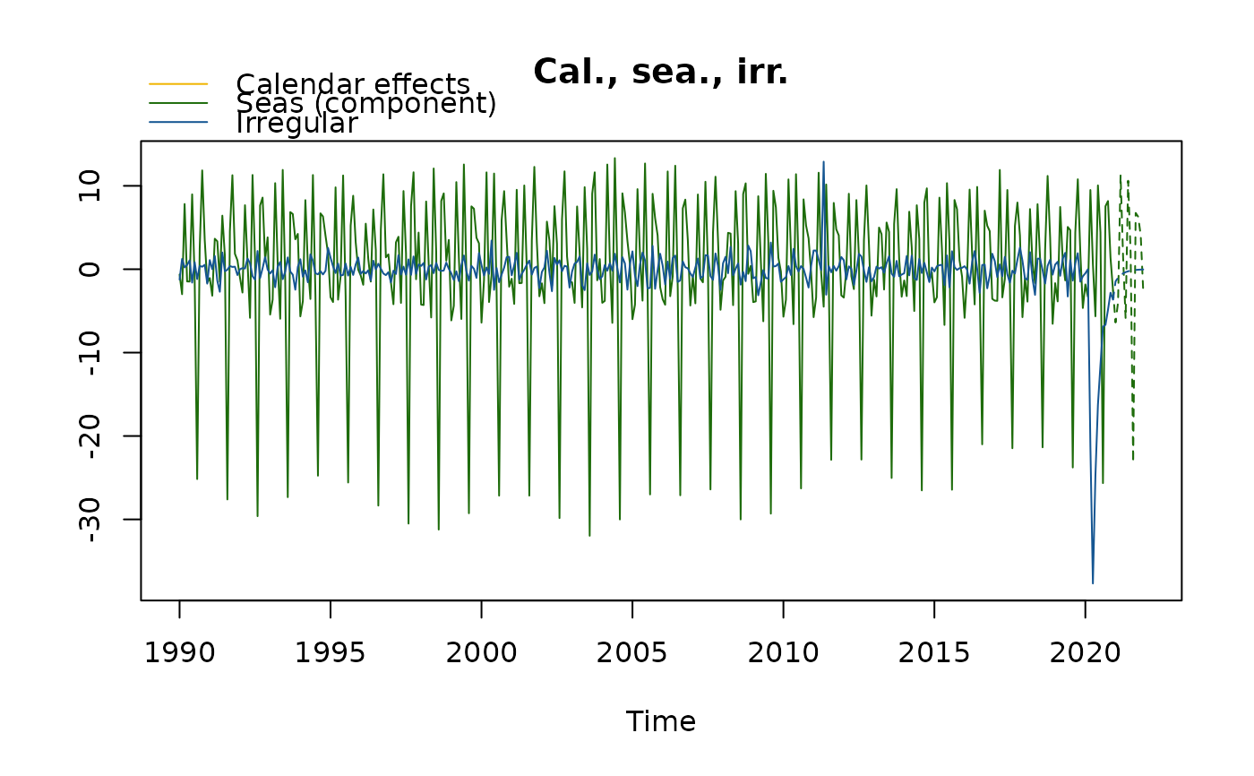
c("final","mts","ts","matrix"). The matrix contains the final results of the seasonal adjustment: the original time series (y)and its forecast (y_f), the trend (t) and its forecast (t_f), the seasonally adjusted series (sa) and its forecast (sa_f), the seasonal component (s)and its forecast (s_f), and the irregular component (i) and its forecast (i_f).- diagnostics
an object of class
"diagnostics", that is a list containing three types of tests results:variance_decompositiona data.frame with the tests results on the relative contribution of the components to the stationary portion of the variance in the original series, after the removal of the long term trend;residuals_testa data.frame with the tests results of the presence of seasonality in the residuals (including the statistic test values, the corresponding p-values and the parameters description);combined_testthe combined tests for stable seasonality in the entire series. The format is a two-element list with:tests_for_stable_seasonality, a data.frame containing the tests results (including the statistic test value, its p-value and the parameters description), andcombined_seasonality_test, the summary.
- user_defined
an object of class
"user_defined": a list containing the additional userdefined variables.
Details
The first step of a seasonal adjustment consists in pre-adjusting the time series with TRAMO. This is done by removing
its deterministic effects (calendar and outliers), using a regression model with ARIMA noise (RegARIMA, see: regarima).
In the second part, the pre-adjusted series is decomposed by the SEATS algorithm into the following components:
trend-cycle (t), seasonal component (s) and irregular component (i). The decomposition can be:
additive (\(y = t + s + i\)) or multiplicative (\(y = t * s * i\), in the latter case pre-adjustment and decomposition are performed
on (\(log(y) = log(t) + log(s) + log(i)\)).
In the TRAMO-SEATS method, the second step - SEATS ("Signal Extraction in ARIMA Time Series") - performs an ARIMA-based decomposition of an observed time series into unobserved components. More information on this method at https://jdemetra-new-documentation.netlify.app/m-seats-decomposition.
The available predefined 'JDemetra+' TRAMO-SEATS model specifications are described in the table below:
| Identifier | | Log/level detection | | Outliers detection | | Calendar effects | | ARIMA | RSA0 | | NA | | NA | |
| NA | | Airline(+mean) | RSA1 | | automatic | | AO/LS/TC | | NA | | Airline(+mean) | RSA2 | |
| automatic | | AO/LS/TC | | 2 td vars + Easter | | Airline(+mean) | RSA3 | | automatic | | AO/LS/TC | | NA | |
| automatic | RSA4 | | automatic | | AO/LS/TC | | 2 td vars + Easter | | automatic | RSA5 | | automatic | |
| AO/LS/TC | | 7 td vars + Easter | | automatic | RSAfull | | automatic | | AO/LS/TC | | automatic | | automatic |
References
More information and examples related to 'JDemetra+' features in the online documentation: https://jdemetra-new-documentation.netlify.app/
BOX G.E.P. and JENKINS G.M. (1970), "Time Series Analysis: Forecasting and Control", Holden-Day, San Francisco.
BOX G.E.P., JENKINS G.M., REINSEL G.C. and LJUNG G.M. (2015), "Time Series Analysis: Forecasting and Control", John Wiley & Sons, Hoboken, N. J., 5th edition.
Examples
# \donttest{
#Example 1
myseries <- ipi_c_eu[, "FR"]
myspec <- tramoseats_spec("RSAfull")
mysa <- tramoseats(myseries, myspec)
mysa
#> RegARIMA
#> y = regression model + arima (2, 1, 0, 0, 1, 1)
#> Log-transformation: no
#> Coefficients:
#> Estimate Std. Error
#> Phi(1) 0.4032 0.051
#> Phi(2) 0.2883 0.051
#> BTheta(1) -0.6641 0.042
#>
#> Estimate Std. Error
#> Week days 0.6994 0.032
#> Leap year 2.3231 0.690
#> Easter [6] -2.5154 0.436
#> AO (5-2011) 13.4679 1.787
#> TC (4-2020) -22.2128 2.205
#> TC (3-2020) -21.0391 2.217
#> AO (5-2000) 6.7386 1.794
#>
#>
#> Residual standard error: 2.326 on 348 degrees of freedom
#> Log likelihood = -816.1, aic = 1654 aicc = 1655, bic(corrected for length) = 1.852
#>
#>
#>
#> Decomposition
#> Model
#> AR : 1 + 0.403230 B + 0.288342 B^2
#> D : 1 - B - B^12 + B^13
#> MA : 1 - 0.664088 B^12
#>
#>
#> SA
#> AR : 1 + 0.403230 B + 0.288342 B^2
#> D : 1 - 2.000000 B + B^2
#> MA : 1 - 0.970348 B + 0.005940 B^2 - 0.005813 B^3 + 0.003576 B^4
#> Innovation variance: 0.7043507
#>
#> Trend
#> D : 1 - 2.000000 B + B^2
#> MA : 1 + 0.033519 B - 0.966481 B^2
#> Innovation variance: 0.06093642
#>
#> Seasonal
#> D : 1 + B + B^2 + B^3 + B^4 + B^5 + B^6 + B^7 + B^8 + B^9 + B^10 + B^11
#> MA : 1 + 1.328957 B + 1.105787 B^2 + 1.185470 B^3 + 1.067845 B^4 + 0.820748 B^5 + 0.632456 B^6 + 0.404457 B^7 + 0.245256 B^8 + 0.001615 B^9 - 0.055617 B^10 - 0.203557 B^11
#> Innovation variance: 0.04290744
#>
#> Transitory
#> AR : 1 + 0.403230 B + 0.288342 B^2
#> MA : 1 - 0.260079 B - 0.739921 B^2
#> Innovation variance: 0.05287028
#>
#> Irregular
#> Innovation variance: 0.2032994
#>
#>
#>
#> Final
#> Last observed values
#> y sa t s i
#> Jan 2020 101.0 102.93775 103.0182 -1.9377453 -0.08043801
#> Feb 2020 100.1 103.53944 103.2312 -3.4394383 0.30818847
#> Mar 2020 91.8 82.47698 103.4998 9.3230241 -21.02286361
#> Apr 2020 66.7 65.77310 103.9608 0.9268969 -38.18766871
#> May 2020 73.7 79.43342 104.7269 -5.7334221 -25.29345247
#> Jun 2020 98.2 88.07766 105.3319 10.1223443 -17.25422206
#> Jul 2020 97.4 92.71048 105.4216 4.6895154 -12.71111705
#> Aug 2020 71.7 97.32129 104.9801 -25.6212858 -7.65880696
#> Sep 2020 104.7 97.44274 104.0807 7.2572622 -6.63793072
#> Oct 2020 106.7 98.20925 103.1711 8.4907485 -4.96183772
#> Nov 2020 101.6 99.98044 102.4813 1.6195550 -2.50088282
#> Dec 2020 96.6 98.99458 101.9735 -2.3945790 -2.97892307
#>
#> Forecasts:
#> y_f sa_f t_f s_f i_f
#> Jan 2021 93.22264 100.1984 101.7578 -6.975740 -1.55946363
#> Feb 2021 96.81455 100.8845 101.7113 -4.069924 -0.82679910
#> Mar 2021 111.72198 100.8668 101.6647 10.855228 -0.79795880
#> Apr 2021 102.76178 101.0716 101.6181 1.690178 -0.54654378
#> May 2021 95.52744 101.2474 101.5716 -5.719910 -0.32422597
#> Jun 2021 111.44221 101.2711 101.5250 10.171157 -0.25395653
#> Jul 2021 103.57813 101.2947 101.4784 2.283395 -0.18370915
#> Aug 2021 78.21363 101.3135 101.4319 -23.099833 -0.11841662
#> Sep 2021 108.57631 101.3000 101.3853 7.276282 -0.08528380
#> Oct 2021 107.32040 101.2771 101.3387 6.043321 -0.06166933
#> Nov 2021 105.33458 101.2505 101.2922 4.084088 -0.04168414
#> Dec 2021 98.79675 101.2164 101.2456 -2.419656 -0.02920922
#>
#>
#> Diagnostics
#> Relative contribution of the components to the stationary
#> portion of the variance in the original series,
#> after the removal of the long term trend
#> Trend computed by Hodrick-Prescott filter (cycle length = 8.0 years)
#> Component
#> Cycle 6.087
#> Seasonal 80.528
#> Irregular 0.965
#> TD & Hol. 3.590
#> Others 8.102
#> Total 99.271
#>
#> Combined test in the entire series
#> Non parametric tests for stable seasonality
#> P.value
#> Kruskall-Wallis test 0.00
#> Test for the presence of seasonality assuming stability 0.00
#> Evolutive seasonality test 0.01
#>
#> Identifiable seasonality present
#>
#> Residual seasonality tests
#> P.value
#> qs test on sa 1.000
#> qs test on i 1.000
#> f-test on sa (seasonal dummies) 1.000
#> f-test on i (seasonal dummies) 1.000
#> Residual seasonality (entire series) 1.000
#> Residual seasonality (last 3 years) 0.974
#> f-test on sa (td) 0.152
#> f-test on i (td) 0.224
#>
#>
#> Additional output variables
# Equivalent to:
mysa1 <- tramoseats(myseries, spec = "RSAfull")
mysa1
#> RegARIMA
#> y = regression model + arima (2, 1, 0, 0, 1, 1)
#> Log-transformation: no
#> Coefficients:
#> Estimate Std. Error
#> Phi(1) 0.4032 0.051
#> Phi(2) 0.2883 0.051
#> BTheta(1) -0.6641 0.042
#>
#> Estimate Std. Error
#> Week days 0.6994 0.032
#> Leap year 2.3231 0.690
#> Easter [6] -2.5154 0.436
#> AO (5-2011) 13.4679 1.787
#> TC (4-2020) -22.2128 2.205
#> TC (3-2020) -21.0391 2.217
#> AO (5-2000) 6.7386 1.794
#>
#>
#> Residual standard error: 2.326 on 348 degrees of freedom
#> Log likelihood = -816.1, aic = 1654 aicc = 1655, bic(corrected for length) = 1.852
#>
#>
#>
#> Decomposition
#> Model
#> AR : 1 + 0.403230 B + 0.288342 B^2
#> D : 1 - B - B^12 + B^13
#> MA : 1 - 0.664088 B^12
#>
#>
#> SA
#> AR : 1 + 0.403230 B + 0.288342 B^2
#> D : 1 - 2.000000 B + B^2
#> MA : 1 - 0.970348 B + 0.005940 B^2 - 0.005813 B^3 + 0.003576 B^4
#> Innovation variance: 0.7043507
#>
#> Trend
#> D : 1 - 2.000000 B + B^2
#> MA : 1 + 0.033519 B - 0.966481 B^2
#> Innovation variance: 0.06093642
#>
#> Seasonal
#> D : 1 + B + B^2 + B^3 + B^4 + B^5 + B^6 + B^7 + B^8 + B^9 + B^10 + B^11
#> MA : 1 + 1.328957 B + 1.105787 B^2 + 1.185470 B^3 + 1.067845 B^4 + 0.820748 B^5 + 0.632456 B^6 + 0.404457 B^7 + 0.245256 B^8 + 0.001615 B^9 - 0.055617 B^10 - 0.203557 B^11
#> Innovation variance: 0.04290744
#>
#> Transitory
#> AR : 1 + 0.403230 B + 0.288342 B^2
#> MA : 1 - 0.260079 B - 0.739921 B^2
#> Innovation variance: 0.05287028
#>
#> Irregular
#> Innovation variance: 0.2032994
#>
#>
#>
#> Final
#> Last observed values
#> y sa t s i
#> Jan 2020 101.0 102.93775 103.0182 -1.9377453 -0.08043801
#> Feb 2020 100.1 103.53944 103.2312 -3.4394383 0.30818847
#> Mar 2020 91.8 82.47698 103.4998 9.3230241 -21.02286361
#> Apr 2020 66.7 65.77310 103.9608 0.9268969 -38.18766871
#> May 2020 73.7 79.43342 104.7269 -5.7334221 -25.29345247
#> Jun 2020 98.2 88.07766 105.3319 10.1223443 -17.25422206
#> Jul 2020 97.4 92.71048 105.4216 4.6895154 -12.71111705
#> Aug 2020 71.7 97.32129 104.9801 -25.6212858 -7.65880696
#> Sep 2020 104.7 97.44274 104.0807 7.2572622 -6.63793072
#> Oct 2020 106.7 98.20925 103.1711 8.4907485 -4.96183772
#> Nov 2020 101.6 99.98044 102.4813 1.6195550 -2.50088282
#> Dec 2020 96.6 98.99458 101.9735 -2.3945790 -2.97892307
#>
#> Forecasts:
#> y_f sa_f t_f s_f i_f
#> Jan 2021 93.22264 100.1984 101.7578 -6.975740 -1.55946363
#> Feb 2021 96.81455 100.8845 101.7113 -4.069924 -0.82679910
#> Mar 2021 111.72198 100.8668 101.6647 10.855228 -0.79795880
#> Apr 2021 102.76178 101.0716 101.6181 1.690178 -0.54654378
#> May 2021 95.52744 101.2474 101.5716 -5.719910 -0.32422597
#> Jun 2021 111.44221 101.2711 101.5250 10.171157 -0.25395653
#> Jul 2021 103.57813 101.2947 101.4784 2.283395 -0.18370915
#> Aug 2021 78.21363 101.3135 101.4319 -23.099833 -0.11841662
#> Sep 2021 108.57631 101.3000 101.3853 7.276282 -0.08528380
#> Oct 2021 107.32040 101.2771 101.3387 6.043321 -0.06166933
#> Nov 2021 105.33458 101.2505 101.2922 4.084088 -0.04168414
#> Dec 2021 98.79675 101.2164 101.2456 -2.419656 -0.02920922
#>
#>
#> Diagnostics
#> Relative contribution of the components to the stationary
#> portion of the variance in the original series,
#> after the removal of the long term trend
#> Trend computed by Hodrick-Prescott filter (cycle length = 8.0 years)
#> Component
#> Cycle 6.087
#> Seasonal 80.528
#> Irregular 0.965
#> TD & Hol. 3.590
#> Others 8.102
#> Total 99.271
#>
#> Combined test in the entire series
#> Non parametric tests for stable seasonality
#> P.value
#> Kruskall-Wallis test 0.00
#> Test for the presence of seasonality assuming stability 0.00
#> Evolutive seasonality test 0.01
#>
#> Identifiable seasonality present
#>
#> Residual seasonality tests
#> P.value
#> qs test on sa 1.000
#> qs test on i 1.000
#> f-test on sa (seasonal dummies) 1.000
#> f-test on i (seasonal dummies) 1.000
#> Residual seasonality (entire series) 1.000
#> Residual seasonality (last 3 years) 0.974
#> f-test on sa (td) 0.152
#> f-test on i (td) 0.224
#>
#>
#> Additional output variables
#Example 2
var1 <- ts(rnorm(length(myseries))*10, start = start(myseries), frequency = 12)
var2 <- ts(rnorm(length(myseries))*100, start = start(myseries), frequency = 12)
var <- ts.union(var1, var2)
myspec2 <- tramoseats_spec(myspec, tradingdays.mauto = "Unused",
tradingdays.option = "WorkingDays",
easter.type = "Standard",
automdl.enabled = FALSE, arima.mu = TRUE,
usrdef.varEnabled = TRUE, usrdef.var = var)
s_preVar(myspec2)
#> $series
#> var1 var2
#> Jan 1990 20.17342464 -35.7620220
#> Feb 1990 11.95608651 -45.4297352
#> Mar 1990 6.56575520 28.6157701
#> Apr 1990 10.26297846 -28.9179390
#> May 1990 5.20192659 51.1904574
#> Jun 1990 11.20615649 -110.4334548
#> Jul 1990 3.99897655 -22.2474789
#> Aug 1990 -9.84527658 -145.2151487
#> Sep 1990 -5.02562184 39.9298770
#> Oct 1990 9.87148440 142.8571193
#> Nov 1990 21.91481010 -48.2140994
#> Dec 1990 -1.65042212 99.2388183
#> Jan 1991 -6.86040800 -116.3700651
#> Feb 1991 9.41399410 162.0789124
#> Mar 1991 -1.64042843 -10.7448152
#> Apr 1991 -13.02339410 -77.3206773
#> May 1991 -7.23484004 -73.6278805
#> Jun 1991 13.90088740 81.5706680
#> Jul 1991 6.81840626 220.3036444
#> Aug 1991 4.68260280 -67.1046628
#> Sep 1991 4.20921089 -42.1589604
#> Oct 1991 -8.00331265 -77.7749125
#> Nov 1991 -4.88457510 56.1542375
#> Dec 1991 5.39004516 -222.2507056
#> Jan 1992 14.35171017 -69.5413671
#> Feb 1992 -2.61838719 -38.3549957
#> Mar 1992 -14.18623721 205.8566983
#> Apr 1992 -5.13792720 -110.7988264
#> May 1992 7.72301225 -95.5938774
#> Jun 1992 14.03682339 -63.5768417
#> Jul 1992 -0.15804912 76.6757452
#> Aug 1992 -10.23289556 68.6958102
#> Sep 1992 -21.16392160 172.1426693
#> Oct 1992 1.50371437 85.1309252
#> Nov 1992 -5.20871198 42.9908280
#> Dec 1992 -9.05454844 -105.5277738
#> Jan 1993 -7.49986903 -4.5880971
#> Feb 1993 -7.86576021 -13.1881384
#> Mar 1993 -5.59681870 -31.9463558
#> Apr 1993 -13.90851305 47.3606163
#> May 1993 -2.82630602 81.2516099
#> Jun 1993 -4.80284997 25.6612328
#> Jul 1993 -9.67621014 -214.8765835
#> Aug 1993 17.77940980 69.0108551
#> Sep 1993 -0.69089037 -177.2443831
#> Oct 1993 -4.26188249 54.6294039
#> Nov 1993 -22.51403727 1.8945820
#> Dec 1993 -9.14170952 -74.8702215
#> Jan 1994 -8.00524582 -79.4321035
#> Feb 1994 -7.53305904 30.0784394
#> Mar 1994 6.60649173 5.4665853
#> Apr 1994 17.27695639 36.4229108
#> May 1994 7.82678579 -116.5186698
#> Jun 1994 -7.81818406 26.0555826
#> Jul 1994 -1.25797549 -241.7116277
#> Aug 1994 10.15236070 114.9085017
#> Sep 1994 2.94676272 120.6579247
#> Oct 1994 -2.96458790 -43.1982134
#> Nov 1994 -8.22289822 10.6856739
#> Dec 1994 16.91546077 48.6195719
#> Jan 1995 -14.76545705 -155.3458324
#> Feb 1995 9.29693563 -108.3142387
#> Mar 1995 -6.13832093 -51.6012028
#> Apr 1995 6.17598091 -20.7770980
#> May 1995 -8.30615177 90.7281411
#> Jun 1995 -11.33375927 81.1425127
#> Jul 1995 -1.56378319 -99.1193254
#> Aug 1995 -2.43091747 -45.4306958
#> Sep 1995 -11.29264413 -31.5728538
#> Oct 1995 -0.62192485 -100.6333083
#> Nov 1995 4.87082631 -101.6594660
#> Dec 1995 -0.54636953 202.9964782
#> Jan 1996 -1.98624209 -68.7638434
#> Feb 1996 -14.53375000 -158.7906854
#> Mar 1996 1.98434624 101.6938102
#> Apr 1996 -13.91001690 -72.3102186
#> May 1996 -22.44235104 -145.3485040
#> Jun 1996 -2.31792440 -214.0815482
#> Jul 1996 -6.86551360 13.4854427
#> Aug 1996 -4.82915280 66.1997776
#> Sep 1996 -22.43508266 49.4613170
#> Oct 1996 -3.81078571 -152.6643655
#> Nov 1996 1.16047733 -11.0216005
#> Dec 1996 8.92492885 246.8741282
#> Jan 1997 18.08520401 -56.3543434
#> Feb 1997 10.79663512 -144.5853422
#> Mar 1997 14.52055280 -47.6555776
#> Apr 1997 25.56923589 101.4600468
#> May 1997 10.72728070 -11.8020034
#> Jun 1997 -11.78914989 -35.4321844
#> Jul 1997 10.75417132 28.7255843
#> Aug 1997 0.53855088 1.8012616
#> Sep 1997 -2.34343833 -89.8423976
#> Oct 1997 9.50759734 144.4736492
#> Nov 1997 0.73021934 -53.7799146
#> Dec 1997 6.63527998 -48.2359998
#> Jan 1998 -8.16198742 -73.5619613
#> Feb 1998 2.95544263 -1.5235256
#> Mar 1998 13.46357662 -28.5060838
#> Apr 1998 -2.80015436 -77.0895994
#> May 1998 -0.63043628 -191.1522944
#> Jun 1998 -1.32833831 17.7899655
#> Jul 1998 6.29361770 19.6320685
#> Aug 1998 -6.41231532 5.0044155
#> Sep 1998 -1.04018599 -104.5274438
#> Oct 1998 -13.88668827 -13.6682386
#> Nov 1998 4.37214206 122.7500609
#> Dec 1998 3.15862087 -19.3865193
#> Jan 1999 1.94610535 -199.3071105
#> Feb 1999 -4.55762127 -42.9905670
#> Mar 1999 8.12534989 -65.1916325
#> Apr 1999 2.75042593 -132.2755316
#> May 1999 0.06009411 -61.1002356
#> Jun 1999 20.10186412 -43.3484772
#> Jul 1999 3.13808823 22.1131620
#> Aug 1999 -8.46162712 41.4635297
#> Sep 1999 -1.34641045 100.3519632
#> Oct 1999 14.70832200 -262.6042237
#> Nov 1999 -14.75125736 -87.3534926
#> Dec 1999 2.04499683 -77.3710833
#> Jan 2000 -3.41768421 59.3058550
#> Feb 2000 18.42157648 45.3563341
#> Mar 2000 -2.05909535 -48.9626711
#> Apr 2000 15.02231278 -66.6085502
#> May 2000 2.42188060 -108.9654228
#> Jun 2000 0.53455720 -104.0906952
#> Jul 2000 -1.25146310 50.1606680
#> Aug 2000 2.47787238 4.1353765
#> Sep 2000 -6.26612578 -5.3081681
#> Oct 2000 6.82877534 -152.7399081
#> Nov 2000 5.89606056 -16.3568520
#> Dec 2000 -8.14967320 -213.5094918
#> Jan 2001 -3.45798987 -13.6833591
#> Feb 2001 0.56529047 -290.4220640
#> Mar 2001 -5.66766181 33.7012645
#> Apr 2001 -0.42837457 76.4510656
#> May 2001 -12.81559297 -66.9378190
#> Jun 2001 9.67582242 -16.0968872
#> Jul 2001 10.29048853 150.7261029
#> Aug 2001 -21.66425254 -12.1693844
#> Sep 2001 -3.03348223 -24.3414776
#> Oct 2001 1.79268039 70.8157194
#> Nov 2001 14.27395820 -48.0039667
#> Dec 2001 -6.19946595 -31.6551268
#> Jan 2002 -1.31842450 51.0471244
#> Feb 2002 2.67551749 -26.6264354
#> Mar 2002 -14.56778518 63.6432097
#> Apr 2002 2.34340520 -101.3955594
#> May 2002 -9.51528054 93.2230747
#> Jun 2002 18.98439401 -65.0788332
#> Jul 2002 -10.42770546 43.6178180
#> Aug 2002 -13.33746286 -16.4089402
#> Sep 2002 17.64724810 126.8656386
#> Oct 2002 5.06063430 41.5432504
#> Nov 2002 -6.55292217 -4.8104283
#> Dec 2002 6.67508839 19.8292951
#> Jan 2003 13.72876146 -38.8687305
#> Feb 2003 5.94581979 -45.2232286
#> Mar 2003 8.09307437 -13.9421427
#> Apr 2003 -9.29351716 -132.5197658
#> May 2003 -9.68882573 75.4069518
#> Jun 2003 -5.63483049 135.7852830
#> Jul 2003 18.88488707 -122.0784861
#> Aug 2003 -1.16769607 -56.7918662
#> Sep 2003 -0.49778439 -118.8849569
#> Oct 2003 4.12530895 -101.2275885
#> Nov 2003 3.39006216 -43.2531486
#> Dec 2003 -2.19463937 34.5706392
#> Jan 2004 -2.79921977 19.0927596
#> Feb 2004 -1.84466622 128.7488578
#> Mar 2004 -11.31041190 -21.3504255
#> Apr 2004 5.99068143 59.3561305
#> May 2004 -3.45024460 -181.5799874
#> Jun 2004 3.28683628 -46.0524573
#> Jul 2004 -0.02001793 74.6337982
#> Aug 2004 -16.43640470 89.8995877
#> Sep 2004 8.30144580 -115.5462161
#> Oct 2004 13.11300782 -28.2423821
#> Nov 2004 -7.25708977 -0.3256871
#> Dec 2004 -3.88345065 151.5028276
#> Jan 2005 -10.42408354 30.9380270
#> Feb 2005 7.39965537 -46.0958821
#> Mar 2005 -3.79227989 29.3447573
#> Apr 2005 8.55040406 7.0972006
#> May 2005 9.29726811 -231.3759365
#> Jun 2005 -5.11420306 19.2706032
#> Jul 2005 5.75606727 -35.2441451
#> Aug 2005 -11.79760738 -153.3292787
#> Sep 2005 8.73922726 -173.4069209
#> Oct 2005 7.52654962 14.1892735
#> Nov 2005 6.31952946 -21.9599601
#> Dec 2005 4.89051671 59.1564494
#> Jan 2006 4.93466172 24.0247909
#> Feb 2006 -20.24668739 -37.2564160
#> Mar 2006 -1.15346633 26.4545865
#> Apr 2006 4.02961199 65.1544488
#> May 2006 -13.29553215 -41.8319774
#> Jun 2006 8.50032275 -207.8760627
#> Jul 2006 11.05681923 59.0955041
#> Aug 2006 4.04141906 -70.5640744
#> Sep 2006 -1.23141511 98.6688400
#> Oct 2006 4.48847720 3.2359045
#> Nov 2006 20.68153748 -49.6043573
#> Dec 2006 -12.49536842 167.3249059
#> Jan 2007 -2.19531175 -105.1266614
#> Feb 2007 10.32002706 2.8015821
#> Mar 2007 -15.82876585 52.6890091
#> Apr 2007 0.84967784 127.0786920
#> May 2007 12.10794619 -58.7592446
#> Jun 2007 -0.23462572 -43.0471444
#> Jul 2007 0.84693918 -2.2966263
#> Aug 2007 -3.25065508 7.4873923
#> Sep 2007 5.05923564 -208.9995616
#> Oct 2007 4.15272046 102.3897173
#> Nov 2007 -11.77413897 62.3240132
#> Dec 2007 0.33445330 -136.7330008
#> Jan 2008 -6.79873381 4.4589523
#> Feb 2008 9.77814031 36.6273799
#> Mar 2008 17.72477385 -17.8469697
#> Apr 2008 2.77933293 210.1677593
#> May 2008 -4.81019306 -24.2409658
#> Jun 2008 -17.91060602 1.1717215
#> Jul 2008 5.30663702 -277.8433689
#> Aug 2008 -11.24766175 27.4491395
#> Sep 2008 0.40226151 -62.2731928
#> Oct 2008 -11.87967396 -102.7831717
#> Nov 2008 22.48831114 72.8990109
#> Dec 2008 15.53161749 -39.2461437
#> Jan 2009 3.23021948 35.7845575
#> Feb 2009 0.22759699 -75.5189860
#> Mar 2009 -2.49427874 6.6689713
#> Apr 2009 -21.72319120 25.7355650
#> May 2009 -13.39659118 -9.0963056
#> Jun 2009 -9.80485754 -73.0508027
#> Jul 2009 -17.92780676 -39.5841246
#> Aug 2009 5.22812809 -141.5808515
#> Sep 2009 -15.91328479 -10.8938918
#> Oct 2009 8.06263133 7.4299910
#> Nov 2009 -6.83813068 45.0190145
#> Dec 2009 3.34388057 38.7345818
#> Jan 2010 9.43006421 -25.8295014
#> Feb 2010 -8.98387674 152.3490603
#> Mar 2010 7.67335868 55.1343438
#> Apr 2010 0.92338676 32.9901773
#> May 2010 -3.51696026 17.2922695
#> Jun 2010 1.15373005 42.6641536
#> Jul 2010 -1.43261353 -81.3699585
#> Aug 2010 -24.19820346 65.1355094
#> Sep 2010 -11.63794035 91.9981796
#> Oct 2010 1.03426653 39.0101788
#> Nov 2010 -1.26143326 95.6724098
#> Dec 2010 -1.41743410 -16.9973563
#> Jan 2011 9.10437035 -37.9977916
#> Feb 2011 14.77617914 14.4207957
#> Mar 2011 16.46242603 -71.8284089
#> Apr 2011 -1.79993025 20.6108648
#> May 2011 9.76856385 -36.7334361
#> Jun 2011 -1.86602735 78.8442877
#> Jul 2011 -0.34098393 -31.0952795
#> Aug 2011 14.88732203 -85.9140099
#> Sep 2011 -1.89839298 108.5279663
#> Oct 2011 -10.89309617 -78.4779324
#> Nov 2011 3.71089482 -122.0960234
#> Dec 2011 -10.27770114 -105.6691432
#> Jan 2012 0.14915848 -99.6890554
#> Feb 2012 -5.20298562 -67.2605085
#> Mar 2012 -0.52244428 66.5268367
#> Apr 2012 -14.35079571 223.6077683
#> May 2012 -3.27979065 -60.1798169
#> Jun 2012 -12.85347619 -29.1617742
#> Jul 2012 -4.25537239 -84.0974862
#> Aug 2012 2.57475661 203.1699515
#> Sep 2012 2.01319396 42.9372125
#> Oct 2012 4.82077401 81.1017521
#> Nov 2012 5.06636590 -17.4299949
#> Dec 2012 -5.26691357 -31.6371483
#> Jan 2013 -5.64773980 -49.3001895
#> Feb 2013 0.40398035 19.0778474
#> Mar 2013 -2.00781380 -110.3744984
#> Apr 2013 -9.04217194 -10.6413314
#> May 2013 1.66655524 145.8992713
#> Jun 2013 -5.24284783 -30.7474298
#> Jul 2013 0.17563903 75.7181411
#> Aug 2013 9.48517187 -171.0825390
#> Sep 2013 2.70265784 59.5309608
#> Oct 2013 -1.60941404 -206.7966650
#> Nov 2013 19.65199507 -8.5739756
#> Dec 2013 3.95548042 3.2286550
#> Jan 2014 8.73719370 28.9686397
#> Feb 2014 4.72324156 80.8938069
#> Mar 2014 -14.85226449 32.6262471
#> Apr 2014 -8.36162299 -170.3857479
#> May 2014 -6.46269212 52.5504589
#> Jun 2014 -0.47437037 -80.3033850
#> Jul 2014 1.67759989 -23.7655721
#> Aug 2014 -0.99738669 85.5349059
#> Sep 2014 0.85996455 -46.9487045
#> Oct 2014 -3.72574031 11.8012784
#> Nov 2014 1.81332543 124.7441555
#> Dec 2014 -9.06806411 -68.8397299
#> Jan 2015 5.91157152 -138.3569575
#> Feb 2015 7.92513233 -4.2932415
#> Mar 2015 0.76872383 -20.9234230
#> Apr 2015 -0.67837199 -146.6993454
#> May 2015 4.33288047 223.5778380
#> Jun 2015 0.49095403 -62.5144963
#> Jul 2015 -0.32800048 -116.7913785
#> Aug 2015 -5.10924776 14.9528831
#> Sep 2015 3.56430539 86.1319900
#> Oct 2015 4.17946136 -104.6203407
#> Nov 2015 5.79205261 17.2260011
#> Dec 2015 -14.75158654 -30.7020751
#> Jan 2016 13.23805231 90.3345610
#> Feb 2016 10.30621466 98.5248694
#> Mar 2016 3.17373893 164.3828484
#> Apr 2016 -11.11903788 81.4559724
#> May 2016 6.21211169 82.5113161
#> Jun 2016 18.09108552 -34.5773922
#> Jul 2016 11.13986006 41.1147335
#> Aug 2016 4.65350534 -64.3214383
#> Sep 2016 -10.68629729 94.2059477
#> Oct 2016 2.55940284 46.9591784
#> Nov 2016 -7.77218934 -66.2112238
#> Dec 2016 -9.50318237 -30.9471102
#> Jan 2017 12.30516332 79.4574264
#> Feb 2017 -2.90321330 -91.4850956
#> Mar 2017 -12.45249585 -46.5520309
#> Apr 2017 -9.25110623 81.9669363
#> May 2017 -3.51758271 152.1035738
#> Jun 2017 -0.41630828 26.5354790
#> Jul 2017 7.29297422 61.9066940
#> Aug 2017 2.93403029 47.1080837
#> Sep 2017 35.86945476 46.3144213
#> Oct 2017 7.55743006 -16.0161363
#> Nov 2017 4.00127303 -3.5685472
#> Dec 2017 8.29345713 -57.4684816
#> Jan 2018 -3.05136243 84.5350017
#> Feb 2018 7.10103322 -58.1766123
#> Mar 2018 4.38613817 -50.2357106
#> Apr 2018 3.58223697 108.8076265
#> May 2018 -1.24237651 -39.2953019
#> Jun 2018 -6.93216085 -66.0461119
#> Jul 2018 5.74346528 -14.9025127
#> Aug 2018 -2.17159515 -87.5485298
#> Sep 2018 30.37581163 169.9001571
#> Oct 2018 -15.91667131 6.8190262
#> Nov 2018 -6.73689236 53.3187580
#> Dec 2018 7.28572805 -8.0948993
#> Jan 2019 -11.51562235 244.6781428
#> Feb 2019 -11.50775213 38.3899034
#> Mar 2019 -1.32075277 -105.2171578
#> Apr 2019 -5.81046358 -172.2233827
#> May 2019 16.61350032 -63.0819250
#> Jun 2019 11.67948978 -95.3595979
#> Jul 2019 7.69885462 -7.9982465
#> Aug 2019 -1.63115808 106.2695902
#> Sep 2019 12.75265346 135.1056836
#> Oct 2019 1.80887984 23.3290220
#> Nov 2019 14.74360522 33.3898791
#> Dec 2019 -15.17434724 -76.4770258
#> Jan 2020 3.04400356 76.9384460
#> Feb 2020 1.07467387 -21.5012961
#> Mar 2020 -12.24792573 38.3380585
#> Apr 2020 4.48519979 -54.2495361
#> May 2020 5.08070951 -209.4578220
#> Jun 2020 3.50212641 37.8050059
#> Jul 2020 7.58213674 -70.5934228
#> Aug 2020 2.90928722 -58.7104530
#> Sep 2020 0.22859592 10.0086359
#> Oct 2020 -2.08143110 120.2066359
#> Nov 2020 -2.63611625 65.9843996
#> Dec 2020 -19.84135796 -62.6745356
#>
#> $description
#> type coeff
#> var1 Undefined NA
#> var2 Undefined NA
#>
mysa2 <- tramoseats(myseries, myspec2,
userdefined = c("decomposition.sa_lin_f",
"decomposition.sa_lin_e"))
mysa2
#> RegARIMA
#> y = regression model + arima (0, 1, 1, 0, 1, 1)
#> Log-transformation: no
#> Coefficients:
#> Estimate Std. Error
#> Theta(1) -0.6286 0.042
#> BTheta(1) -0.6720 0.042
#>
#> Estimate Std. Error
#> Mean 1.244e-03 0.016
#> r.var1 2.513e-02 0.011
#> r.var2 -8.779e-04 0.001
#> Monday 6.495e-01 0.240
#> Tuesday 8.164e-01 0.239
#> Wednesday 1.071e+00 0.239
#> Thursday 3.325e-02 0.239
#> Friday 9.035e-01 0.241
#> Saturday -1.591e+00 0.238
#> Leap year 2.124e+00 0.723
#> Easter [6] -2.164e+00 0.483
#> TC (4-2020) -2.166e+01 2.220
#> TC (3-2020) -2.094e+01 2.208
#> AO (5-2011) 1.267e+01 1.902
#> LS (11-2008) -1.290e+01 1.639
#>
#>
#> Residual standard error: 2.222 on 341 degrees of freedom
#> Log likelihood = -800, aic = 1636 aicc = 1638, bic(corrected for length) = 1.876
#>
#>
#>
#> Decomposition
#> Model
#> D : 1 - B - B^12 + B^13
#> MA : 1 - 0.628618 B - 0.671952 B^12 + 0.422401 B^13
#>
#>
#> SA
#> D : 1 - 2.000000 B + B^2
#> MA : 1 - 1.598990 B + 0.610996 B^2
#> Innovation variance: 0.71507
#>
#> Trend
#> D : 1 - 2.000000 B + B^2
#> MA : 1 + 0.032502 B - 0.967498 B^2
#> Innovation variance: 0.02439346
#>
#> Seasonal
#> D : 1 + B + B^2 + B^3 + B^4 + B^5 + B^6 + B^7 + B^8 + B^9 + B^10 + B^11
#> MA : 1 + 0.828663 B + 0.585037 B^2 + 0.320734 B^3 + 0.070806 B^4 - 0.142616 B^5 - 0.307533 B^6 - 0.419888 B^7 - 0.481876 B^8 - 0.500824 B^9 - 0.488831 B^10 - 0.463674 B^11
#> Innovation variance: 0.03127962
#>
#> Irregular
#> Innovation variance: 0.4605053
#>
#>
#>
#> Final
#> Last observed values
#> y sa t s i
#> Jan 2020 101.0 102.78062 103.3134 -1.780621 -0.53273175
#> Feb 2020 100.1 103.45777 103.4134 -3.357770 0.04432381
#> Mar 2020 91.8 82.37178 103.5479 9.428222 -21.17610817
#> Apr 2020 66.7 66.02583 103.7774 0.674173 -37.75153471
#> May 2020 73.7 79.35820 104.1323 -5.658197 -24.77408258
#> Jun 2020 98.2 88.08398 104.4185 10.116020 -16.33452920
#> Jul 2020 97.4 92.95224 104.4724 4.447759 -11.52018771
#> Aug 2020 71.7 97.37303 104.2600 -25.673032 -6.88700314
#> Sep 2020 104.7 97.15478 103.8402 7.545219 -6.68546102
#> Oct 2020 106.7 98.52972 103.4167 8.170279 -4.88695561
#> Nov 2020 101.6 100.21515 103.0788 1.384854 -2.86370217
#> Dec 2020 96.6 99.17476 102.8398 -2.574762 -3.66506567
#>
#> Forecasts:
#> y_f sa_f t_f s_f i_f
#> Jan 2021 95.14843 101.2900 102.7554 -6.427888 -1.46540458
#> Feb 2021 98.01290 101.7259 102.7517 -3.928320 -1.02578320
#> Mar 2021 113.62435 102.0300 102.7480 11.264885 -0.71804824
#> Apr 2021 104.00158 102.2419 102.7445 1.530754 -0.50263377
#> May 2021 96.53854 102.3893 102.7411 -5.887663 -0.35184364
#> Jun 2021 113.19844 102.4916 102.7379 10.600718 -0.24629055
#> Jul 2021 104.43242 102.5623 102.7347 1.839560 -0.17240338
#> Aug 2021 79.61642 102.6110 102.7316 -23.182854 -0.12068237
#> Sep 2021 109.42362 102.6442 102.7287 6.761079 -0.08447766
#> Oct 2021 109.20290 102.6667 102.7259 6.246391 -0.05913436
#> Nov 2021 106.96640 102.6818 102.7232 4.093091 -0.04139405
#> Dec 2021 100.56264 102.6916 102.7206 -2.537114 -0.02897584
#>
#>
#> Diagnostics
#> Relative contribution of the components to the stationary
#> portion of the variance in the original series,
#> after the removal of the long term trend
#> Trend computed by Hodrick-Prescott filter (cycle length = 8.0 years)
#> Component
#> Cycle 1.760
#> Seasonal 57.870
#> Irregular 0.997
#> TD & Hol. 2.532
#> Others 35.139
#> Total 98.299
#>
#> Combined test in the entire series
#> Non parametric tests for stable seasonality
#> P.value
#> Kruskall-Wallis test 0.000
#> Test for the presence of seasonality assuming stability 0.000
#> Evolutive seasonality test 0.064
#>
#> Identifiable seasonality present
#>
#> Residual seasonality tests
#> P.value
#> qs test on sa 1.000
#> qs test on i 1.000
#> f-test on sa (seasonal dummies) 1.000
#> f-test on i (seasonal dummies) 1.000
#> Residual seasonality (entire series) 1.000
#> Residual seasonality (last 3 years) 0.960
#> f-test on sa (td) 0.958
#> f-test on i (td) 1.000
#>
#>
#> Additional output variables
#> Names of additional variables (2):
#> decomposition.sa_lin_f, decomposition.sa_lin_e
plot(mysa2)
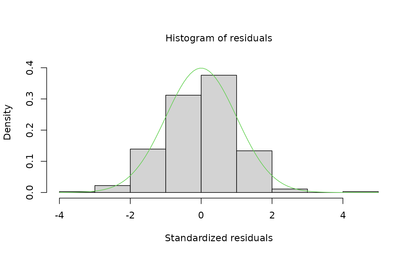
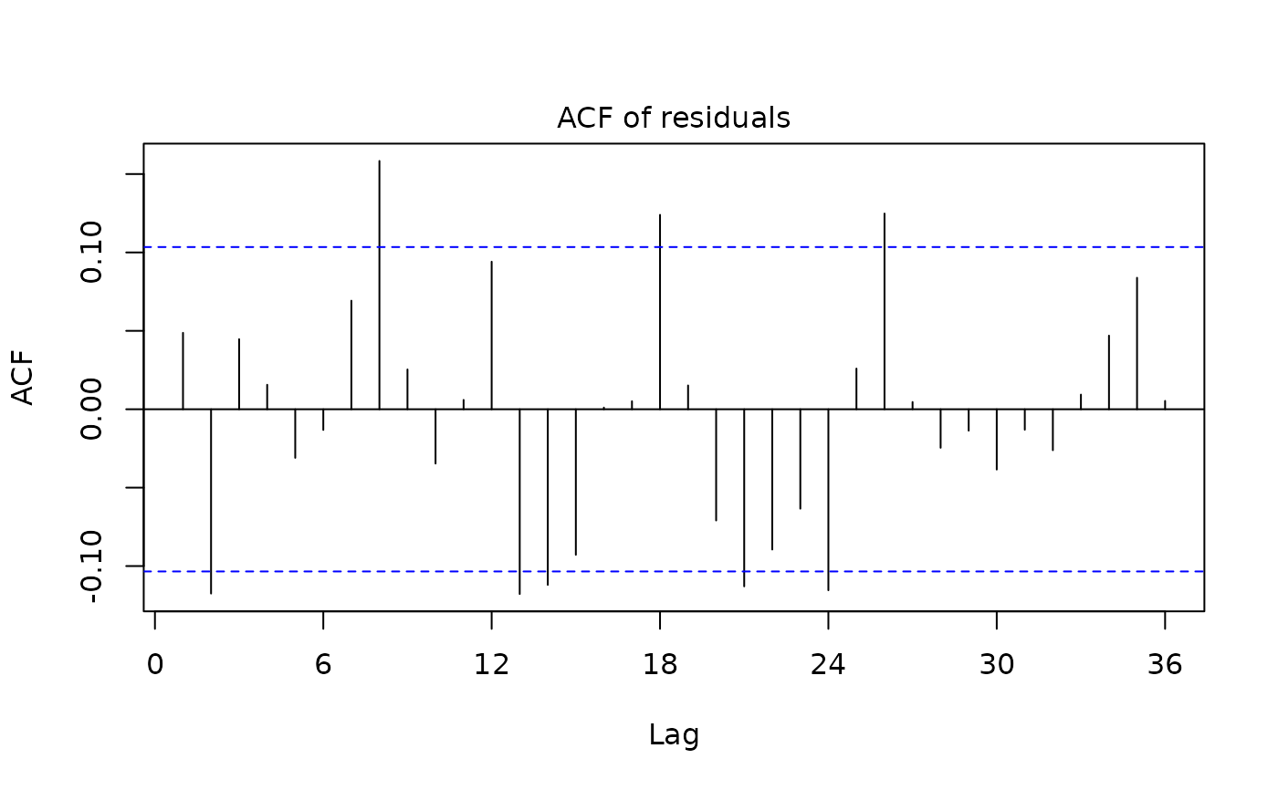
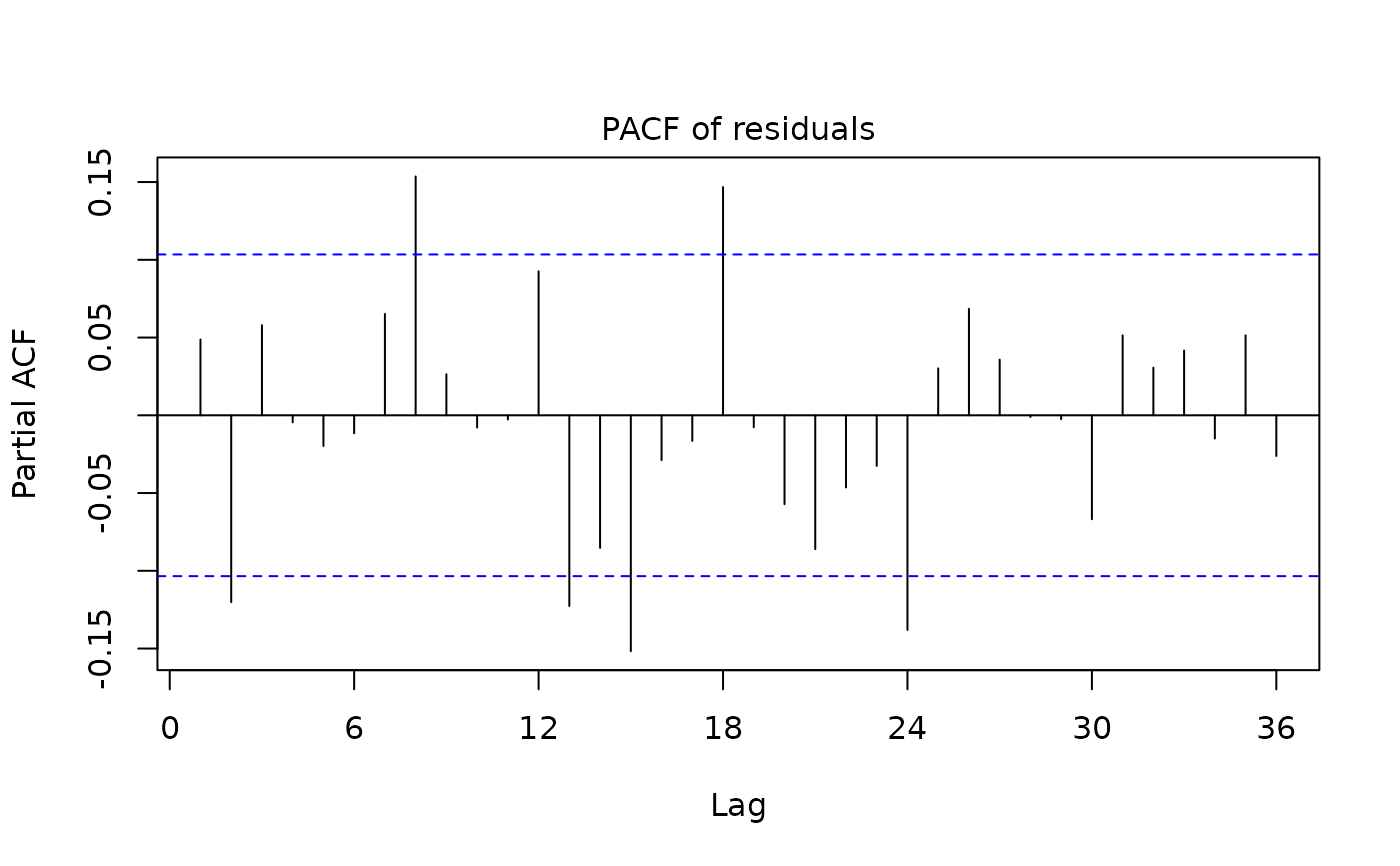
 plot(mysa2$regarima)


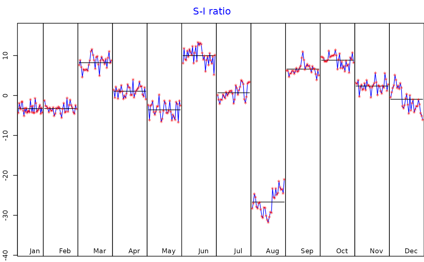
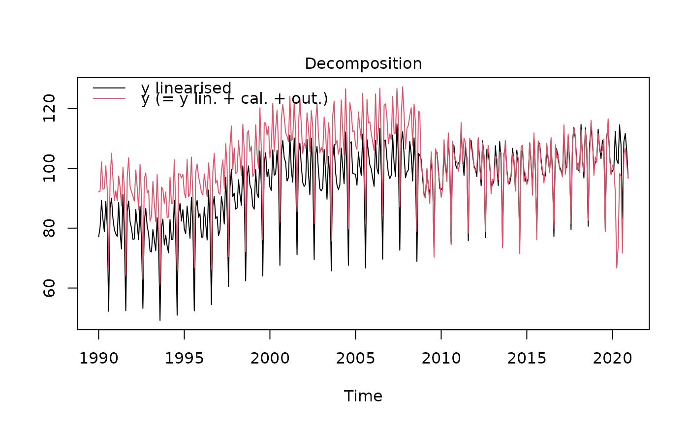 plot(mysa2$decomposition)
 # }
# }